Tutorials
Networks
In this exercise, we will explore networks and distance. We will start by using an abstract network of points and lines to illustrate some concepts, and then move on to using real-world data to identify proximate objects based on network distance.
Import libraries
import geopandas as gpd
import numpy as np
import matplotlib.pyplot as plt
from shapely.geometry import LineString, MultiLineString, Point, Polygon
import pandas as pd
import requests
import networkx as nx
import osmnx as ox
import h3
import libpysal as lps
We’ll import our helper library and update the graph output just like in the previous tutorial.
from cdptools import utilsutils.set_axis_off()To begin, we will find the approximate bounding box of NYC.
# bounding box of nyc
bbox = (-74.3, 40.5, -73.7, 40.9)
Create random network
We’ll begin by creating a dataframe of 100 random points. As we can see below, we are using numpy to generate random numbers, along with geopandas’ points_from_xy() to create a geodataframe from these points. We are using the bounds of NYC to make sure that the network approximately covers the city.
# create a geodataframe of 100 random points
np.random.seed(0)
n = 100
df = pd.DataFrame(
    {
        "geometry": gpd.points_from_xy(
            np.random.uniform(-74.3, -73.7, n),
            np.random.uniform(40.5, 40.9, n),
        ),
    }
)
And here we cast the dataframe as a geodataframe and set its CRS.
gdf = gpd.GeoDataFrame(df, crs="EPSG:4326")As we can see from our initial plot, we have a mass of 100 randomly distributed points. At this stage, this is meaningless!
gdf.plot()<Axes: >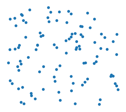
Since we are creating a network (instead of analyzing an already existing one), let’s connect each node to its five nearest neighbors (measured based on straight-line or Euclidean distance). We’ll use geopandas’ distance method to calculate the distance between each pair of points, and then use that to create a list of edges. There are many ways to calculate distance like this, some of which are more appropriate for working with a greater volume of data (scipy’s KDTree operations chief among them).
We can also ignore the warning about the geographic CRS as well given our use case and scale, but do keep in mind that projection-related considerations are extremely important when calculating distances.
# find five nearest neighbors for each point, not including itself
k = 5
neighbors = gdf.geometry.apply(lambda x: gdf.geometry.distance(x)).values.argsort(
    axis=1
)[:, 1 : k + 1]

# join neighbors to original dataframe
gdf["neighbors"] = neighbors.tolist()
/var/folders/g5/b592wl6x12s0tx4jfw9f7_j40000gn/T/ipykernel_49295/2007509322.py:3: UserWarning: Geometry is in a geographic CRS. Results from 'distance' are likely incorrect. Use 'GeoSeries.to_crs()' to re-project geometries to a projected CRS before this operation.
neighbors = gdf.geometry.apply(lambda x: gdf.geometry.distance(x)).values.argsort(gdf.neighbors0 [12, 28, 88, 2, 37]
1 [83, 91, 42, 39, 31]
2 [88, 12, 62, 37, 0]
3 [84, 11, 22, 51, 56]
4 [29, 41, 32, 58, 80]
...
95 [61, 24, 57, 87, 15]
96 [33, 50, 91, 83, 1]
97 [75, 69, 67, 15, 92]
98 [66, 8, 52, 72, 1]
99 [15, 34, 67, 61, 82]
Name: neighbors, Length: 100, dtype: objectNow if we inspect our dataframe, we see that we have an additional column, neighbors, which contains the row index number of the five nearest points to that row.
gdf.head(5)| geometry | neighbors | |
|---|---|---|
| 0 | POINT (-73.97071 40.77113) | [12, 28, 88, 2, 37] |
| 1 | POINT (-73.87089 40.608) | [83, 91, 42, 39, 31] |
| 2 | POINT (-73.93834 40.79408) | [88, 12, 62, 37, 0] |
| 3 | POINT (-73.97307 40.88488) | [84, 11, 22, 51, 56] |
| 4 | POINT (-74.04581 40.5995) | [29, 41, 32, 58, 80] |
Based on that information, we can now draw lines (or network edges) between each point and its nearest neighbors. We can use the following function to create an array of lines between a point and it’s neighbors.
Let’s consider the component parts of the function:
lines = []: we create an empty array to store line geometry infor i, neighbor in enumerage(r.neighbors): we set up aforloop to iterate through each row’s list of point indexeslines.append(LineString([r.geometry, gdf.loc[neighbor].geometry])): we create a newLineStringgeometry with two points: the starting point at the input rowr.geometry, and ending at the looked up neighbor’s geometrygdf.loc[neighbor].geometry. The.loc[neighbor]allows us to find the row that matches based on the neighborid, and then we access itsgeometrypropertyreturn MultiLineString(lines): we combine each of the line geometries in thelinesarray into one complexMultiLineString, which is what it sounds like (a combination ofLineStrings).
def create_lines(r):
    lines = []
    for i, neighbor in enumerate(r.neighbors):
        lines.append(LineString([r.geometry, gdf.loc[neighbor].geometry]))
    return MultiLineString(lines)
We can then apply the function to each row (axis=1). Keep in mind that when executing a function via apply(), the row (or column) input is implied and is the default input r in the function.
gdf["line_geometry"] = gdf.apply(create_lines, axis=1)If we inspect our dataframe again, we’ll see a new column line_geometry which represents the edges between each point and its five nearest neighbors.
gdf.head()| geometry | neighbors | line_geometry | |
|---|---|---|---|
| 0 | POINT (-73.97071 40.77113) | [12, 28, 88, 2, 37] | MULTILINESTRING ((-73.97071 40.77113, -73.9591... |
| 1 | POINT (-73.87089 40.608) | [83, 91, 42, 39, 31] | MULTILINESTRING ((-73.87089 40.608, -73.88452 ... |
| 2 | POINT (-73.93834 40.79408) | [88, 12, 62, 37, 0] | MULTILINESTRING ((-73.93834 40.79408, -73.9544... |
| 3 | POINT (-73.97307 40.88488) | [84, 11, 22, 51, 56] | MULTILINESTRING ((-73.97307 40.88488, -73.9600... |
| 4 | POINT (-74.04581 40.5995) | [29, 41, 32, 58, 80] | MULTILINESTRING ((-74.04581 40.5995, -74.0512 ... |
We can create a new geodataframe based on this edges geometry and plot it- now we have a connected network of points and lines!
lines_gdf = gpd.GeoDataFrame(
    gdf[["line_geometry"]], geometry="line_geometry", crs="EPSG:4326"
)
ax = lines_gdf.plot(color="black", alpha=0.5, linewidth=0.2)
gdf.plot(ax=ax, color="black")
# optionally save the figure to file
# plt.savefig("lines.pdf", bbox_inches="tight", pad_inches=0)<Axes: >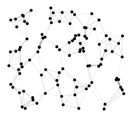
Saving our datasets
You may optionally want to save these nodes and edges to file to inspect in QGIS or another software. To do so, we use the to_file() function to save out as GeoJSON files
gdf["geometry"].to_file("nodes.geojson", driver="GeoJSON")
gdf["line_geometry"].to_file("edges.geojson", driver="GeoJSON")
/Users/marioag/miniforge3/envs/cdp26/lib/python3.14/site-packages/pyogrio/geopandas.py:917: UserWarning: 'crs' was not provided. The output dataset will not have projection information defined and may not be usable in other systems.
write(gdf.sample(10)| geometry | neighbors | line_geometry | |
|---|---|---|---|
| 91 | POINT (-73.89955 40.58394) | [83, 1, 96, 50, 33] | MULTILINESTRING ((-73.89955 40.58394, -73.8845... |
| 29 | POINT (-74.0512 40.61603) | [4, 41, 58, 32, 90] | MULTILINESTRING ((-74.0512 40.61603, -74.04581... |
| 2 | POINT (-73.93834 40.79408) | [88, 12, 62, 37, 0] | MULTILINESTRING ((-73.93834 40.79408, -73.9544... |
| 50 | POINT (-73.95788 40.55978) | [96, 73, 33, 91, 32] | MULTILINESTRING ((-73.95788 40.55978, -73.9480... |
| 44 | POINT (-73.89994 40.82248) | [56, 62, 45, 74, 2] | MULTILINESTRING ((-73.89994 40.82248, -73.9081... |
| 78 | POINT (-74.12232 40.78177) | [48, 94, 30, 85, 57] | MULTILINESTRING ((-74.12232 40.78177, -74.1107... |
| 33 | POINT (-73.95894 40.61931) | [96, 50, 91, 58, 83] | MULTILINESTRING ((-73.95894 40.61931, -73.9480... |
| 65 | POINT (-74.07876 40.84232) | [40, 9, 51, 49, 48] | MULTILINESTRING ((-74.07876 40.84232, -74.0843... |
| 75 | POINT (-74.27649 40.58957) | [97, 69, 92, 67, 15] | MULTILINESTRING ((-74.27649 40.58957, -74.2879... |
| 45 | POINT (-73.89762 40.78156) | [62, 37, 44, 2, 56] | MULTILINESTRING ((-73.89762 40.78156, -73.9062... |
Let’s plot the nearest neighbors and connecting edges for a single point. Below, we take a random point s and then highlight it in blue, and connect it to its five nearest neighbors in orange. Keep in mind that every time you rerun the following cell, a new sampled point will be chosen.
# plot the lines for a single point
s = gdf.sample()
ax = lines_gdf.plot(color="black", alpha=0.5, linewidth=0.2)
gdf.plot(ax=ax, color="red")

s.plot(ax=ax, color="blue")
gpd.GeoSeries(s.line_geometry).plot(ax=plt.gca(), color="orange")
<Axes: >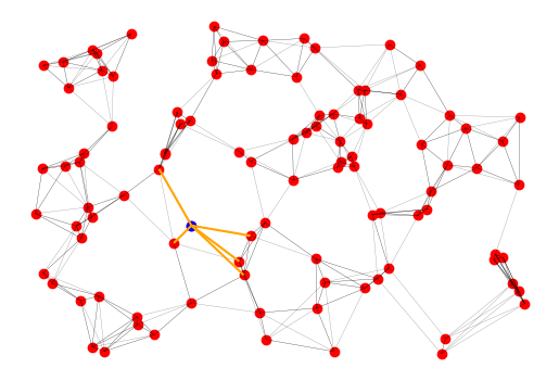
Apply to a real-world example
The toy problem above was a fine way to explore this concept, so now let’s apply it to real-world networks. We will use an API endpoint hosted through catalog.data.gov to find MTA subway stations in NYC.
There are a couple of things to keep in mind about the following API request. First is the request itself: we use the popular requests library to perform a GET request (there are many types of requests, read more here) on the API endpoint listed at the resource URL.
We can see on the open data portal’s website that the dataset has the option to download as JSON: :

Get subway stations in NYC
If a query is successful, it will return a result that starts with 2**, such as 200. Error codes are reserved for 4** and 5**. We can make this most basic request first to confirm that our query is properly formatted:
requests.get("https://data.ny.gov/api/v3/views/39hk-dx4f/query.json?accessType=API")<Response [200]>What we really want, however, is the json associated with the response. We can create a new variable and set it to equal the response json payload:
subway_stations = requests.get(
    "https://data.ny.gov/api/v3/views/39hk-dx4f/query.json?accessType=API"
).json()
If we print the results, we see we have an array of objects (up to 2000) that represents the restaurants in MN09. If you scan through, you’ll see attributes like street, building number, cuisine_description, and restaurant scores.
For these to be useful to us, let’s cast the array as a geodataframe. Take a look at the resulting subway_stations JSON object to see how to translate the geometry into a geodataframe. Remember, we need to extract the lat and lon of the geometry JSON to pass to geopandas.
subway_stations[0]{':id': 'row-3523-2f4j~u7nt',
':version': 'rv-sw7x-24xf.jkj9',
':created_at': '2026-07-24T04:15:49.117Z',
':updated_at': '2026-07-24T04:15:53.449Z',
'gtfs_stop_id': 'R01',
'station_id': '1',
'complex_id': '1',
'division': 'BMT',
'line': 'Astoria',
'stop_name': 'Astoria-Ditmars Blvd',
'borough': 'Q',
'cbd': 'false',
'daytime_routes': 'N W',
'structure': 'Elevated',
'gtfs_latitude': '40.775036',
'gtfs_longitude': '-73.912034',
'north_direction_label': 'Last Stop',
'south_direction_label': 'Manhattan',
'ada': '0',
'ada_northbound': '0',
'ada_southbound': '0',
'georeference': {'type': 'Point', 'coordinates': [-73.912034, 40.775036]},
':@computed_region_yamh_8v7k': '196',
':@computed_region_wbg7_3whc': '877',
':@computed_region_kjdx_g34t': '2137'}subway_stations = gpd.GeoDataFrame(
subway_stations,
geometry=gpd.points_from_xy(
[x["georeference"]["coordinates"][0] for x in subway_stations],
[x["georeference"]["coordinates"][1] for x in subway_stations],
),
)subway_stations.fillna("na", inplace=True)| :id | :version | :created_at | :updated_at | gtfs_stop_id | station_id | complex_id | division | line | stop_name | ... | south_direction_label | ada | ada_northbound | ada_southbound | georeference | :@computed_region_yamh_8v7k | :@computed_region_wbg7_3whc | :@computed_region_kjdx_g34t | ada_notes | geometry | |
|---|---|---|---|---|---|---|---|---|---|---|---|---|---|---|---|---|---|---|---|---|---|
| 0 | row-3523-2f4j~u7nt | rv-sw7x-24xf.jkj9 | 2026-07-24T04:15:49.117Z | 2026-07-24T04:15:53.449Z | R01 | 1 | 1 | BMT | Astoria | Astoria-Ditmars Blvd | ... | Manhattan | 0 | 0 | 0 | {'type': 'Point', 'coordinates': [-73.912034, ... | 196 | 877 | 2137 | na | POINT (-73.91203 40.77504) |
| 1 | row-8siw.4xgw.nvqe | rv-8v4h.spb5-xbnx | 2026-07-24T04:15:49.117Z | 2026-07-24T04:15:53.449Z | R03 | 2 | 2 | BMT | Astoria | Astoria Blvd | ... | Manhattan | 1 | 1 | 1 | {'type': 'Point', 'coordinates': [-73.917843, ... | 196 | 874 | 2137 | na | POINT (-73.91784 40.77026) |
| 2 | row-javd~wecq_zsff | rv-hdit_cfci~5ax6 | 2026-07-24T04:15:49.117Z | 2026-07-24T04:15:53.449Z | R04 | 3 | 3 | BMT | Astoria | 30 Av | ... | Manhattan | 0 | 0 | 0 | {'type': 'Point', 'coordinates': [-73.921479, ... | 196 | 874 | 2137 | na | POINT (-73.92148 40.76678) |
| 3 | row-2e8r~ajpw~63ju | rv-z7ah_qf9a-57cz | 2026-07-24T04:15:49.117Z | 2026-07-24T04:15:53.449Z | R05 | 4 | 4 | BMT | Astoria | Broadway | ... | Manhattan | 0 | 0 | 0 | {'type': 'Point', 'coordinates': [-73.925508, ... | 196 | 878 | 2137 | na | POINT (-73.92551 40.76182) |
| 4 | row-ryyi.7fna_gkrz | rv-t4wf_rwe3-pwsg | 2026-07-24T04:15:49.117Z | 2026-07-24T04:15:53.449Z | R06 | 5 | 5 | BMT | Astoria | 36 Av | ... | Manhattan | 0 | 0 | 0 | {'type': 'Point', 'coordinates': [-73.929575, ... | 196 | 878 | 2137 | na | POINT (-73.92958 40.7568) |
| ... | ... | ... | ... | ... | ... | ... | ... | ... | ... | ... | ... | ... | ... | ... | ... | ... | ... | ... | ... | ... | ... |
| 491 | row-h3sh~q368~ka2u | rv-yqdw~fkiw_5tan | 2026-07-24T04:15:49.117Z | 2026-07-24T04:15:53.449Z | S15 | 517 | 517 | SIR | Staten Island | Prince's Bay | ... | South Shore | 0 | 0 | 0 | {'type': 'Point', 'coordinates': [-74.200064, ... | 585 | 612 | 2139 | na | POINT (-74.20006 40.52551) |
| 492 | row-32hc-iewi-f2ek | rv-np3s_geps_e4i3 | 2026-07-24T04:15:49.117Z | 2026-07-24T04:15:53.449Z | S14 | 518 | 518 | SIR | Staten Island | Pleasant Plains | ... | South Shore | 0 | 0 | 0 | {'type': 'Point', 'coordinates': [-74.217847, ... | 585 | 612 | 2139 | na | POINT (-74.21785 40.52241) |
| 493 | row-gp6r-gwsn~hpj7 | rv-k536.6x6e~fxx5 | 2026-07-24T04:15:49.117Z | 2026-07-24T04:15:53.449Z | S13 | 519 | 519 | SIR | Staten Island | Richmond Valley | ... | Tottenville | 0 | 0 | 0 | {'type': 'Point', 'coordinates': [-74.229141, ... | 585 | 612 | 2139 | na | POINT (-74.22914 40.51963) |
| 494 | row-s585-gppp.cqqf | rv-xs6u_ne9t.8mpv | 2026-07-24T04:15:49.117Z | 2026-07-24T04:15:53.449Z | S09 | 522 | 522 | SIR | Staten Island | Tottenville | ... | Last Stop | 1 | 1 | 1 | {'type': 'Point', 'coordinates': [-74.251961, ... | 585 | 610 | na | na | POINT (-74.25196 40.51276) |
| 495 | row-3cih~5yyh~akab | rv-6t5z~swwg.fy9b | 2026-07-24T04:15:49.117Z | 2026-07-24T04:15:53.449Z | S11 | 523 | 523 | SIR | Staten Island | Arthur Kill | ... | Tottenville | 1 | 1 | 1 | {'type': 'Point', 'coordinates': [-74.242096, ... | 585 | 610 | 2139 | na | POINT (-74.2421 40.51658) |
496 rows × 27 columns
Now we can see that we have a dataframe with a number of columns, including a geometry column, that we can use to perform calculations on.
subway_stations.plot()<Axes: >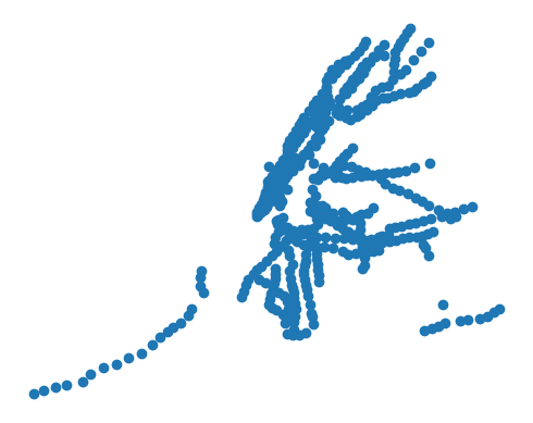
Let’s inspect the number of stations by borough:
subway_stations.borough.value_counts()borough
Bk 169
M 153
Q 83
Bx 70
SI 21
Name: count, dtype: int64Additionally, let’s check out the distribution of ADA accessibility in each borough (0=not accessible, 1=fully accessible, 2=partially accessible):
subway_stations.groupby("borough")["ada"].value_counts()borough ada
Bk 0 124
1 43
2 2
Bx 0 49
1 21
M 0 83
1 64
2 6
Q 0 54
1 28
2 1
SI 0 15
1 6
Name: count, dtype: int64We can also see the distribution of stations in each borough based on their level of accessibility:
subway_stations.groupby("borough")["ada"].value_counts().div(
    subway_stations.groupby("borough")["ada"].count(), level="borough"
)  # expressed as proportions
borough ada
Bk 0 0.733728
1 0.254438
2 0.011834
Bx 0 0.700000
1 0.300000
M 0 0.542484
1 0.418301
2 0.039216
Q 0 0.650602
1 0.337349
2 0.012048
SI 0 0.714286
1 0.285714
dtype: float64Build a graph to allow us to search
Now that we have a geodataframe of subway stations, let’s create a network based on the street grid of the neighborhood around a random station. To do so, we’ll use the total geographic bounds of our restaurants dataframe to request a network from the OSMnx module. OSMnx is built on top of the Networkx library, and makes it easy for users to access information from OpenStreetMap for use in network analysis.
Like the name implies, we can build a network graph from the bbox above using the graph_from_bbox() function. We can specify that we are interested in a walk type network (i.e. pedestrian paths and sidewalks) using the network_type parameter (vs driving or all for example).
Note too that the order of coordinates returned from the total_bounds property does not match the order that OSMnx expects it, so we have to reorder them via the bbox parameter.
sample_station = subway_stations.sample(1)subway_stations[subway_stations.line == "Crosstown"].stop_name.unique()<ArrowStringArray>
[ 'Court Sq', '21 St', 'Greenpoint Av',
'Nassau Av', 'Metropolitan Av', 'Broadway',
'Flushing Av', 'Myrtle-Willoughby Avs', 'Bedford-Nostrand Avs',
'Classon Av', 'Clinton-Washington Avs', 'Fulton St']
Length: 12, dtype: strmy_stop = subway_stations[subway_stations.stop_name == "Bedford-Nostrand Avs"]my_stop| :id | :version | :created_at | :updated_at | gtfs_stop_id | station_id | complex_id | division | line | stop_name | ... | south_direction_label | ada | ada_northbound | ada_southbound | georeference | :@computed_region_yamh_8v7k | :@computed_region_wbg7_3whc | :@computed_region_kjdx_g34t | ada_notes | geometry | |
|---|---|---|---|---|---|---|---|---|---|---|---|---|---|---|---|---|---|---|---|---|---|
| 289 | row-d2ki_njq5-3svz | rv-h2ut.pjne_dxbs | 2026-07-24T04:15:49.117Z | 2026-07-24T04:15:53.449Z | G33 | 289 | 289 | IND | Crosstown | Bedford-Nostrand Avs | ... | Southbound | 0 | 0 | 0 | {'type': 'Point', 'coordinates': [-73.953522, ... | 894 | 883 | 2090 | na | POINT (-73.95352 40.68963) |
1 rows × 27 columns
point_network = ox.graph_from_point(
    (my_stop.iloc[0].geometry.y, my_stop.iloc[0].geometry.x),
    dist=1000,
    network_type="walk",
)
We can confirm that the result is a networkx multidirectional (MultiDiGraph) graph object:
point_network…and we can extract the nodes and edges of that network out as geodataframes:
net_nodes, net_edges = ox.graph_to_gdfs(point_network)ax = net_edges.plot(color="black")
net_nodes.plot(ax=ax, color="blue")
sample_station.plot(ax=ax, color="red")<Axes: >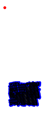
By inspecting the results, we can see that each row is a street network segment with a number of properties, all derived from OSM data.
net_edges.head()| osmid | highway | oneway | reversed | length | name | geometry | service | access | tunnel | |||
|---|---|---|---|---|---|---|---|---|---|---|---|---|
| u | v | key | ||||||||||
| 42492309 | 9833655058 | 0 | 244967357 | service | False | True | 10.829684 | NaN | LINESTRING (-73.96375 40.69209, -73.96378 40.6... | NaN | NaN | NaN |
| 42492312 | 13568945328 | 0 | 40956094 | service | False | False | 8.518390 | Emerson Place | LINESTRING (-73.9619 40.6923, -73.96189 40.69222) | NaN | NaN | NaN |
| 498897281 | 13568945328 | 0 | 40956094 | service | False | True | 1.793625 | Emerson Place | LINESTRING (-73.96188 40.69221, -73.96189 40.6... | NaN | NaN | NaN |
| 504044405 | 9833654949 | 0 | 240737263 | service | False | False | 7.734980 | NaN | LINESTRING (-73.96452 40.68986, -73.9645 40.68... | NaN | NaN | NaN |
| 597728150 | 5912637789 | 0 | 452280723 | pedestrian | False | False | 10.061691 | Underhill Avenue | LINESTRING (-73.96454 40.68108, -73.96456 40.6... | NaN | NaN | NaN |
We can take a look at the distribution of restaurants relative to our network by plotting both:
sample_station| :id | :version | :created_at | :updated_at | gtfs_stop_id | station_id | complex_id | division | line | stop_name | ... | south_direction_label | ada | ada_northbound | ada_southbound | georeference | :@computed_region_yamh_8v7k | :@computed_region_wbg7_3whc | :@computed_region_kjdx_g34t | ada_notes | geometry | |
|---|---|---|---|---|---|---|---|---|---|---|---|---|---|---|---|---|---|---|---|---|---|
| 275 | row-ud6m_efi9_rs6w | rv-rgc5.6tf9~j4p4 | 2026-07-24T04:15:49.117Z | 2026-07-24T04:15:53.449Z | F11 | 275 | 612 | IND | Queens Blvd | Lexington Av/53 St | ... | Downtown | 1 | 1 | 1 | {'type': 'Point', 'coordinates': [-73.969055, ... | 749 | 749 | 2095 | na | POINT (-73.96906 40.75755) |
1 rows × 27 columns
ax = my_stop.plot()
net_edges.plot(ax=ax, color="black", linewidth=0.1)
<Axes: >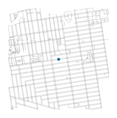
Let’s take a look at the output- we can see a network of nodes and edges that represent the area around our sampled station. Note that unlike our toy example above, network edges here can have corners and curves and are not just individual line segments.
ax = net_edges.plot(color="black", linewidth=0.1, figsize=(10, 10))
net_nodes.plot(ax=ax, color="orange", markersize=1).set_axis_off()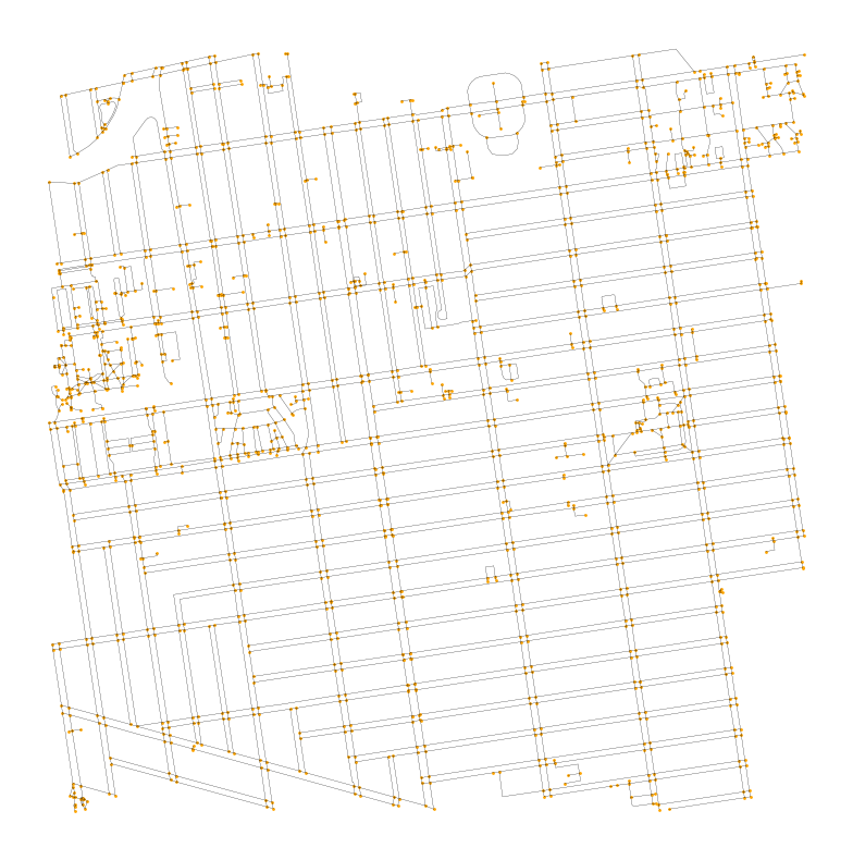
Great - now that we have a network and locations to traverse, let’s get a point to travel to/from.
Get directions to a random point
random_point = net_nodes.sample(1)violins = gpd.GeoDataFrame(geometry=[Point(40.6864252, -73.9598445)], crs="EPSG:4326")First we need to associate our starting point and target points to our networks. We begin by finding the nearest network nodes between an input coordinate and the network, for both our origin and a randomly selected restaurant.
orig = ox.distance.nearest_nodes(point_network, violins.geometry.x, violins.geometry.y)[
    0
]
dest = ox.distance.nearest_nodes(
    point_network, my_stop.iloc[0].geometry.x, my_stop.iloc[0].geometry.y
)
The above functions return the indices of the nearest network nodes:
orig, dest(np.int64(9804257913), 10536943420)Now that we have network positions, we can traverse the network to find the shortest path between each point. To do so, we’ll use the shortest_path() function, and specify our weight as the length between start and end points. There are a number of options for weight, including the number of segments that need to be traversed, or a custom input you specify.
OSMnx also has special helper functions to plot routes, which we’ll use to plot the network and path between points.
# find the shortest path between nodes, minimizing travel distance, then plot it
route = ox.shortest_path(point_network, orig, dest, weight="length")
fig, ax = ox.plot_graph_route(point_network, route, node_size=10)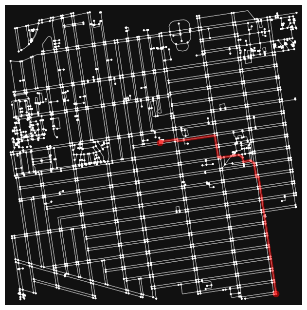
If we inspect the route on its own, we’ll see an array of node ids that are ordered based on the shortest path that is generated.
route[np.int64(9804257913),
9804257916,
9804258118,
9804258121,
9804258153,
9758475742,
9265224809,
9265224803,
9758475744,
9804257488,
9811007575,
9811007532,
9811007533,
9811007501,
10617184513,
9811007502,
9811007485,
9811007486,
9811007469,
9811007470,
9811007453,
9811007454,
9811007176,
9811006945,
9811007204,
9811007201,
5211448859,
5211448871,
5211448870,
5211448868,
5211448867,
5211448873,
1275778444,
1275778398,
5211448872,
9811007028,
10114114529,
9820781453,
9811007041,
9811007038,
9811007056,
9820781474,
9820781475,
9820781477,
9820781472,
10536943419,
10536943422,
10536943420]That’s not super useful to us- thankfully OSMnx makes it easy to convert the route to a geodataframe for use elsewhere. We can also use some basic math to convert the path from meters to miles to put things in perspective.
edge_lengths = ox.routing.route_to_gdf(point_network, route)["length"]

# convert meters to miles
sum(edge_lengths) / 1609.341.1118201423936316def distance_from_point(row, origin):
"""
Returns the distance in miles and the geometry of the shortest path between a point and a destination.
Parameters:
row (pd.Series): A row from a pandas DataFrame.
origin (int): The origin node in the network.
"""
dest = ox.distance.nearest_nodes(point_network, row.geometry.x, row.geometry.y)
route = ox.shortest_path(point_network, origin, dest, weight="length")
edge_lengths = ox.routing.route_to_gdf(point_network, route)["length"]
route_geom = ox.routing.route_to_gdf(point_network, route)
route_geom = route_geom.geometry.union_all()
return {"distance": sum(edge_lengths) / 1609.34, "route_geom": route_geom}sample_station.loc[:, "distance_to_point"] = sample_station.apply(
distance_from_point, origin=orig, axis=1
)If we observe our results, we can see that each row (e.g. each pizza restaurant) has a dictionary of distance in miles and the shortest path. Pretty neat, but not super ergonomic in its current form.
sample_station["distance_to_point"]275 {'distance': 1.9781084301036134, 'route_geom':...
Name: distance_to_point, dtype: objectWe can explode each dictionary key:value pair into a separate column using the below operation. We are combining three different steps in the below cell to achieve this:
- converting the entries in the
distance_from_classattribute into apd.Series- this is what does the separating into separate columns dropping thedistance_from_classfield, as we no longer need it- using the
concat(...)function to concatenate the results of the other two operations; this allows us to combine things back together into our one dataframe
# explode the dictionary into separate columns
sample_station = pd.concat(
    [
        sample_station.drop(["distance_to_point"], axis=1),
        sample_station["distance_to_point"].apply(pd.Series),
    ],
    axis=1,
)
Now we can see we have each of the dictionary entries as new columns, and now we can operate over both in our dataframe.
sample_station.head()| :id | :version | :created_at | :updated_at | gtfs_stop_id | station_id | complex_id | division | line | stop_name | ... | ada_northbound | ada_southbound | georeference | :@computed_region_yamh_8v7k | :@computed_region_wbg7_3whc | :@computed_region_kjdx_g34t | ada_notes | geometry | distance | route_geom | |
|---|---|---|---|---|---|---|---|---|---|---|---|---|---|---|---|---|---|---|---|---|---|
| 275 | row-ud6m_efi9_rs6w | rv-rgc5.6tf9~j4p4 | 2026-07-24T04:15:49.117Z | 2026-07-24T04:15:53.449Z | F11 | 275 | 612 | IND | Queens Blvd | Lexington Av/53 St | ... | 1 | 1 | {'type': 'Point', 'coordinates': [-73.969055, ... | 749 | 749 | 2095 | na | POINT (-73.96906 40.75755) | 1.978108 | MULTILINESTRING ((-73.9433561 40.6809908, -73.... |
1 rows × 29 columns
Now let’s cast our results to a new geodataframe with the geometry set as the routes calculated above.
sample_station_routes = gpd.GeoDataFrame(
    sample_station, geometry="route_geom", crs="EPSG:4326"
)
Now we can plot each pizza restaurant, the shortest path between here and there, and can symbolize based on the distance in miles:
import contextily as cxax = sample_station.plot(color="black", figsize=(10, 10))
sample_station_routes.plot(column="distance", cmap="magma", ax=ax, linewidth=3)
sample_station.plot(column="distance", cmap="magma", legend=True, ax=ax)
cx.add_basemap(ax, crs="EPSG:4326", source=cx.providers.CartoDB.Voyager)
# title
plt.title(
f"Distance from point to subway station: {round(sample_station['distance'].min(), 2)} mi"
)Text(0.5, 1.0, 'Distance from point to subway station: 1.98 mi')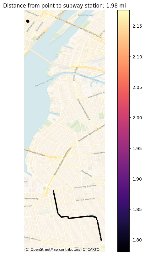
Great- we can now visualize and intuit the closest pizza places. If we want to look at the actual numbers, we can sort by distance and observe. Note that the top two entries are tied, which suggest that both were snapped to the same network node (which is a consideration to keep in mind when we rely on third-party datasets like OSM)
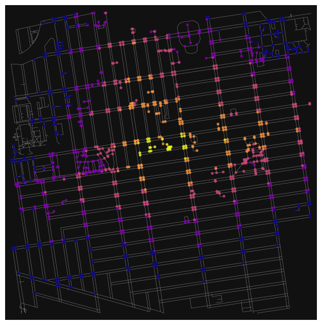
Calculating walksheds
network_type = "walk"
trip_times = [5, 10, 15, 20, 25]  # in minutes
travel_speed = 4.5  # walking speed in km/hour
iso_colors = ox.plot.get_colors(n=len(trip_times), cmap="plasma", start=0)# color the nodes according to isochrone then plot the street network
nodes_outside = []
node_colors = {}
for trip_time, color in zip(sorted(trip_times, reverse=True), iso_colors, strict=False):
subgraph = nx.ego_graph(point_network, dest, radius=trip_time, distance="time")
for node in subgraph.nodes():
node_colors[node] = color
nc = [node_colors.get(node, "none") for node in point_network.nodes()]
ns = [15 if node in node_colors else 0 for node in point_network.nodes()]
nodes_outside.extend(
[node for node in point_network.nodes() if node not in node_colors]
)
nodes_outside = list(set(nodes_outside))
fig, ax = ox.plot.plot_graph(
point_network,
node_color=nc,
node_size=ns,
node_alpha=0.8,
edge_linewidth=0.2,
edge_color="#999999",
)
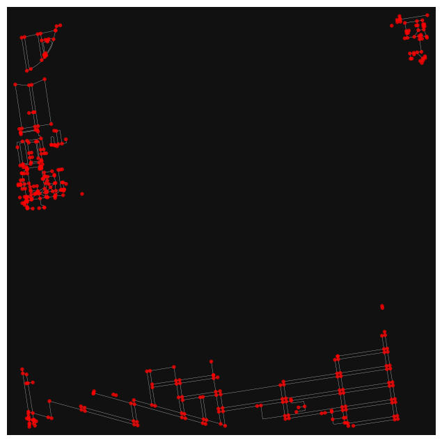
# plot nodes outside walkzone
nodes_outside_graph = point_network.subgraph(nodes_outside)
fig, ax = ox.plot.plot_graph(
    nodes_outside_graph,
    node_color="red",
    node_size=15,
    node_alpha=0.8,
    edge_linewidth=0.2,
    edge_color="#999999",
)
walkzone = requests.get(
    "https://api.mapbox.com/isochrone/v1/mapbox/driving/-118.22258,33.99038?contours_minutes=5,10,15&contours_colors=6706ce,04e813,4286f4&polygons=true&access_token=pk.eyJ1IjoibWdpYW1waWVyaSIsImEiOiJaQ1VSbEdnIn0.sOtbImYVm_Pq682-5mDJEA"
).json()walkzone{'features': [{'properties': {'fill-opacity': 0.33,
'fillColor': '#4286f4',
'opacity': 0.33,
'fill': '#4286f4',
'fillOpacity': 0.33,
'color': '#4286f4',
'contour': 15,
'metric': 'time'},
'geometry': {'coordinates': [[[-118.21958, 34.046974],
[-118.221068, 34.04538],
[-118.221138, 34.043938],
[-118.222384, 34.043184],
[-118.222008, 34.04038],
[-118.22258, 34.039632],
[-118.223994, 34.039966],
[-118.224507, 34.041453],
[-118.22558, 34.041037],
[-118.22658, 34.042128],
[-118.227218, 34.042018],
[-118.227422, 34.04138],
[-118.227021, 34.03938],
[-118.22758, 34.03897],
[-118.229978, 34.038982],
[-118.23258, 34.040518],
[-118.232782, 34.03938],
[-118.23358, 34.038626],
[-118.23458, 34.038924],
[-118.237905, 34.03838],
[-118.234839, 34.038121],
[-118.23458, 34.03643],
[-118.233908, 34.037708],
[-118.233113, 34.03738],
[-118.23358, 34.036402],
[-118.23458, 34.036317],
[-118.235199, 34.034999],
[-118.236492, 34.03438],
[-118.235108, 34.032852],
[-118.23558, 34.031797],
[-118.23658, 34.031702],
[-118.237701, 34.032259],
[-118.23858, 34.035632],
[-118.240096, 34.029896],
[-118.241078, 34.029882],
[-118.24358, 34.032802],
[-118.244852, 34.03238],
[-118.244376, 34.031176],
[-118.24558, 34.029647],
[-118.24958, 34.028713],
[-118.250161, 34.027961],
[-118.252211, 34.02738],
[-118.252726, 34.026526],
[-118.25358, 34.026797],
[-118.255092, 34.02638],
[-118.253671, 34.024289],
[-118.253613, 34.02138],
[-118.25439, 34.02019],
[-118.255095, 34.019895],
[-118.25758, 34.020211],
[-118.257766, 34.01938],
[-118.256911, 34.019049],
[-118.255659, 34.01738],
[-118.256412, 34.016212],
[-118.257934, 34.014734],
[-118.259712, 34.014512],
[-118.26058, 34.013995],
[-118.26158, 34.014194],
[-118.262, 34.01338],
[-118.26085, 34.01238],
[-118.262186, 34.01138],
[-118.262201, 34.01038],
[-118.26358, 34.009703],
[-118.265581, 34.010381],
[-118.267443, 34.00838],
[-118.266703, 34.00738],
[-118.267091, 34.006891],
[-118.26858, 34.006496],
[-118.269129, 34.006831],
[-118.26958, 34.008199],
[-118.271234, 34.006034],
[-118.27258, 34.005481],
[-118.274003, 34.00338],
[-118.27358, 34.002604],
[-118.27258, 34.002777],
[-118.271213, 34.001747],
[-118.269861, 33.99938],
[-118.27258, 33.996552],
[-118.27358, 33.996456],
[-118.278071, 33.99338],
[-118.280803, 33.989603],
[-118.281475, 33.98938],
[-118.279944, 33.989016],
[-118.27885, 33.98738],
[-118.27858, 33.986054],
[-118.27758, 33.985936],
[-118.276586, 33.98438],
[-118.276561, 33.98338],
[-118.27798, 33.98238],
[-118.271335, 33.97738],
[-118.270334, 33.97638],
[-118.270105, 33.97538],
[-118.26858, 33.974177],
[-118.26758, 33.973562],
[-118.26658, 33.97349],
[-118.26558, 33.972017],
[-118.26458, 33.971919],
[-118.26158, 33.969909],
[-118.260449, 33.96738],
[-118.258858, 33.96638],
[-118.25658, 33.962491],
[-118.255558, 33.96338],
[-118.25458, 33.96524],
[-118.25358, 33.962708],
[-118.25258, 33.963527],
[-118.248199, 33.962761],
[-118.248187, 33.960987],
[-118.24858, 33.960542],
[-118.250037, 33.96038],
[-118.248283, 33.959677],
[-118.24758, 33.957212],
[-118.245941, 33.95938],
[-118.244553, 33.960407],
[-118.242301, 33.959659],
[-118.241759, 33.95838],
[-118.240482, 33.957478],
[-118.23958, 33.956174],
[-118.23858, 33.95656],
[-118.23758, 33.954521],
[-118.236283, 33.95638],
[-118.235303, 33.956657],
[-118.23466, 33.95438],
[-118.235031, 33.953831],
[-118.236923, 33.953723],
[-118.237095, 33.95338],
[-118.23558, 33.952075],
[-118.234632, 33.952432],
[-118.2338, 33.95216],
[-118.231101, 33.949859],
[-118.230373, 33.94838],
[-118.22858, 33.947293],
[-118.228283, 33.948677],
[-118.228663, 33.949463],
[-118.22758, 33.951725],
[-118.226896, 33.951696],
[-118.225199, 33.95038],
[-118.225123, 33.94938],
[-118.226018, 33.94838],
[-118.226268, 33.94638],
[-118.22558, 33.946108],
[-118.223727, 33.94638],
[-118.221259, 33.94938],
[-118.21958, 33.950396],
[-118.21758, 33.948052],
[-118.21658, 33.948517],
[-118.21558, 33.949767],
[-118.214516, 33.948444],
[-118.214924, 33.94738],
[-118.21358, 33.945275],
[-118.21058, 33.949061],
[-118.20658, 33.950451],
[-118.204626, 33.952426],
[-118.202404, 33.95338],
[-118.203156, 33.95438],
[-118.20314, 33.95538],
[-118.20258, 33.956019],
[-118.201897, 33.95538],
[-118.20158, 33.954111],
[-118.20058, 33.955542],
[-118.19758, 33.955077],
[-118.19658, 33.953164],
[-118.195863, 33.955663],
[-118.192861, 33.95638],
[-118.194892, 33.957068],
[-118.19458, 33.958103],
[-118.193437, 33.958237],
[-118.19258, 33.959375],
[-118.191761, 33.959561],
[-118.19058, 33.958648],
[-118.189318, 33.958642],
[-118.189171, 33.957971],
[-118.189919, 33.95738],
[-118.185875, 33.956085],
[-118.18558, 33.955229],
[-118.184259, 33.955059],
[-118.183651, 33.95538],
[-118.184687, 33.95638],
[-118.183923, 33.95938],
[-118.181151, 33.96038],
[-118.18478, 33.96238],
[-118.183296, 33.96338],
[-118.18458, 33.963667],
[-118.185322, 33.96438],
[-118.18458, 33.964861],
[-118.18258, 33.965082],
[-118.182001, 33.964959],
[-118.181651, 33.964309],
[-118.18058, 33.964383],
[-118.180195, 33.96538],
[-118.181757, 33.96638],
[-118.17958, 33.967342],
[-118.17858, 33.96669],
[-118.176798, 33.968598],
[-118.17521, 33.96901],
[-118.17502, 33.96938],
[-118.17558, 33.970073],
[-118.17658, 33.969825],
[-118.176934, 33.970734],
[-118.17658, 33.971135],
[-118.17558, 33.970715],
[-118.17458, 33.971301],
[-118.172698, 33.97338],
[-118.17058, 33.974533],
[-118.16958, 33.976],
[-118.168199, 33.97438],
[-118.169039, 33.97338],
[-118.168742, 33.969542],
[-118.16965, 33.96745],
[-118.168668, 33.967292],
[-118.16858, 33.965969],
[-118.168465, 33.967265],
[-118.167324, 33.96738],
[-118.167069, 33.96838],
[-118.167377, 33.97038],
[-118.166902, 33.974702],
[-118.16658, 33.975177],
[-118.165553, 33.97538],
[-118.16658, 33.975927],
[-118.166966, 33.976994],
[-118.166714, 33.98138],
[-118.167187, 33.982773],
[-118.168034, 33.98338],
[-118.16758, 33.98395],
[-118.166202, 33.983758],
[-118.16558, 33.982955],
[-118.164536, 33.983424],
[-118.164073, 33.982887],
[-118.164096, 33.981896],
[-118.165355, 33.98138],
[-118.163437, 33.98038],
[-118.164125, 33.97938],
[-118.16358, 33.978449],
[-118.16158, 33.980126],
[-118.16054, 33.98038],
[-118.161993, 33.981967],
[-118.161928, 33.982728],
[-118.158357, 33.98338],
[-118.159333, 33.98438],
[-118.15758, 33.984918],
[-118.15658, 33.983796],
[-118.15558, 33.984973],
[-118.15458, 33.984239],
[-118.15158, 33.98385],
[-118.149627, 33.98438],
[-118.15058, 33.984875],
[-118.150773, 33.984573],
[-118.152161, 33.984799],
[-118.15358, 33.986732],
[-118.15458, 33.985753],
[-118.15658, 33.98642],
[-118.157311, 33.98738],
[-118.15758, 33.988773],
[-118.15858, 33.98744],
[-118.159581, 33.987381],
[-118.160315, 33.98838],
[-118.158736, 33.98938],
[-118.16058, 33.989874],
[-118.160818, 33.990618],
[-118.155258, 33.99138],
[-118.15858, 33.992144],
[-118.15958, 33.991726],
[-118.160004, 33.991956],
[-118.16058, 33.995781],
[-118.160631, 33.995431],
[-118.16358, 33.995215],
[-118.16458, 33.996018],
[-118.166782, 33.996178],
[-118.166042, 33.99838],
[-118.16719, 33.99938],
[-118.166848, 34.000648],
[-118.165259, 34.000701],
[-118.16458, 33.999732],
[-118.16358, 33.999473],
[-118.160518, 33.999318],
[-118.159965, 33.999765],
[-118.159572, 34.00138],
[-118.159969, 34.001991],
[-118.160433, 34.002527],
[-118.162855, 34.00338],
[-118.16258, 34.00379],
[-118.16158, 34.003903],
[-118.15958, 34.003544],
[-118.158348, 34.00438],
[-118.159833, 34.005127],
[-118.160067, 34.005893],
[-118.159895, 34.006695],
[-118.158664, 34.007464],
[-118.158448, 34.008248],
[-118.15858, 34.008598],
[-118.16058, 34.008816],
[-118.162674, 34.008474],
[-118.16358, 34.007891],
[-118.16758, 34.007643],
[-118.16858, 34.006813],
[-118.169617, 34.007343],
[-118.17158, 34.006521],
[-118.172287, 34.01038],
[-118.172239, 34.015039],
[-118.17185, 34.01765],
[-118.17158, 34.01821],
[-118.170467, 34.01838],
[-118.170384, 34.019184],
[-118.171915, 34.021045],
[-118.172481, 34.027479],
[-118.17258, 34.02754],
[-118.172882, 34.02238],
[-118.17358, 34.021719],
[-118.174296, 34.018096],
[-118.174966, 34.017994],
[-118.17558, 34.018697],
[-118.178543, 34.018417],
[-118.178735, 34.01938],
[-118.17859, 34.01837],
[-118.176017, 34.017943],
[-118.175729, 34.017231],
[-118.17458, 34.017076],
[-118.173168, 34.015792],
[-118.172919, 34.01038],
[-118.17358, 34.007726],
[-118.17758, 34.007746],
[-118.178084, 34.00838],
[-118.177507, 34.00938],
[-118.178145, 34.009815],
[-118.18358, 34.010062],
[-118.1839, 34.0107],
[-118.18266, 34.01138],
[-118.183377, 34.011583],
[-118.191715, 34.012245],
[-118.19158, 34.012949],
[-118.190583, 34.01338],
[-118.192037, 34.013923],
[-118.191983, 34.015783],
[-118.191129, 34.015831],
[-118.19058, 34.014747],
[-118.189907, 34.015707],
[-118.189175, 34.015785],
[-118.18758, 34.014615],
[-118.18558, 34.016013],
[-118.18458, 34.0161],
[-118.18422, 34.01638],
[-118.18458, 34.016972],
[-118.184755, 34.016555],
[-118.186109, 34.016851],
[-118.186439, 34.018239],
[-118.183211, 34.02038],
[-118.19058, 34.021521],
[-118.19258, 34.023911],
[-118.193079, 34.023879],
[-118.19402, 34.02282],
[-118.194597, 34.021397],
[-118.197129, 34.021831],
[-118.197393, 34.02238],
[-118.197259, 34.024059],
[-118.19558, 34.024835],
[-118.19458, 34.024177],
[-118.193854, 34.02438],
[-118.19444, 34.02452],
[-118.194434, 34.025526],
[-118.196085, 34.02738],
[-118.196589, 34.029389],
[-118.19358, 34.029749],
[-118.19258, 34.030729],
[-118.18558, 34.03105],
[-118.18258, 34.030793],
[-118.18158, 34.031102],
[-118.18058, 34.028709],
[-118.180315, 34.032115],
[-118.178578, 34.033378],
[-118.17158, 34.034162],
[-118.170864, 34.034096],
[-118.17058, 34.033092],
[-118.170027, 34.034827],
[-118.168744, 34.03538],
[-118.169461, 34.035499],
[-118.16958, 34.039606],
[-118.169836, 34.035636],
[-118.17458, 34.03561],
[-118.175885, 34.034685],
[-118.17958, 34.034715],
[-118.18058, 34.033797],
[-118.182001, 34.033801],
[-118.18258, 34.033205],
[-118.18458, 34.033049],
[-118.18558, 34.031787],
[-118.194522, 34.03238],
[-118.19515, 34.03638],
[-118.19558, 34.036733],
[-118.19876, 34.03538],
[-118.19958, 34.033529],
[-118.20158, 34.033527],
[-118.203496, 34.032296],
[-118.204744, 34.032216],
[-118.20558, 34.033767],
[-118.20623, 34.03303],
[-118.20758, 34.033232],
[-118.209229, 34.036731],
[-118.21058, 34.0368],
[-118.211372, 34.03738],
[-118.21058, 34.039157],
[-118.208488, 34.03938],
[-118.208895, 34.040065],
[-118.209635, 34.040325],
[-118.209399, 34.041199],
[-118.210104, 34.042856],
[-118.21058, 34.043303],
[-118.211578, 34.042378],
[-118.21258, 34.042546],
[-118.21458, 34.04125],
[-118.215944, 34.04338],
[-118.21558, 34.045051],
[-118.215812, 34.044612],
[-118.21758, 34.0443],
[-118.21958, 34.046974]]],
'type': 'Polygon'},
'type': 'Feature'},
{'properties': {'fill-opacity': 0.33,
'fillColor': '#04e813',
'opacity': 0.33,
'fill': '#04e813',
'fillOpacity': 0.33,
'color': '#04e813',
'contour': 10,
'metric': 'time'},
'geometry': {'coordinates': [[[-118.21958, 34.026469],
[-118.22058, 34.025486],
[-118.222139, 34.02538],
[-118.222323, 34.02438],
[-118.223476, 34.02338],
[-118.222108, 34.02138],
[-118.223061, 34.02038],
[-118.223053, 34.01938],
[-118.22217, 34.01838],
[-118.22258, 34.017996],
[-118.223893, 34.018067],
[-118.22458, 34.018754],
[-118.226145, 34.017945],
[-118.226973, 34.017987],
[-118.227841, 34.02038],
[-118.229817, 34.023143],
[-118.23058, 34.023522],
[-118.23251, 34.02138],
[-118.231848, 34.021112],
[-118.23158, 34.020082],
[-118.233046, 34.01938],
[-118.231831, 34.019129],
[-118.23118, 34.01778],
[-118.23192, 34.01572],
[-118.232903, 34.015703],
[-118.23358, 34.014936],
[-118.23458, 34.015816],
[-118.23558, 34.015091],
[-118.23658, 34.015627],
[-118.237145, 34.014945],
[-118.238119, 34.014841],
[-118.23884, 34.01538],
[-118.23958, 34.017225],
[-118.240332, 34.016132],
[-118.241527, 34.01538],
[-118.24083, 34.01513],
[-118.240255, 34.013055],
[-118.241332, 34.01238],
[-118.24158, 34.011285],
[-118.24258, 34.012865],
[-118.243262, 34.009062],
[-118.244922, 34.009038],
[-118.24558, 34.009706],
[-118.246067, 34.008867],
[-118.247072, 34.00838],
[-118.245271, 34.00738],
[-118.24477, 34.00638],
[-118.24658, 34.005916],
[-118.24758, 34.006538],
[-118.248131, 34.00538],
[-118.251022, 34.00438],
[-118.249199, 34.00238],
[-118.25158, 33.998946],
[-118.25258, 33.999458],
[-118.254615, 33.99638],
[-118.253169, 33.995791],
[-118.253236, 33.995036],
[-118.25458, 33.99496],
[-118.25658, 33.994136],
[-118.25858, 33.992001],
[-118.259368, 33.99038],
[-118.26058, 33.990809],
[-118.261078, 33.989878],
[-118.262327, 33.989633],
[-118.26258, 33.990049],
[-118.26304, 33.98938],
[-118.26058, 33.98874],
[-118.25958, 33.989065],
[-118.258213, 33.988747],
[-118.257825, 33.98838],
[-118.258029, 33.987829],
[-118.258816, 33.98738],
[-118.257341, 33.986619],
[-118.257484, 33.98538],
[-118.25658, 33.98464],
[-118.25358, 33.983827],
[-118.253308, 33.98238],
[-118.2519, 33.98106],
[-118.25058, 33.981247],
[-118.250059, 33.980901],
[-118.24958, 33.979634],
[-118.24658, 33.976898],
[-118.24558, 33.974994],
[-118.24458, 33.975641],
[-118.24158, 33.973007],
[-118.240921, 33.974721],
[-118.238175, 33.974975],
[-118.23758, 33.975518],
[-118.237488, 33.974472],
[-118.23558, 33.973721],
[-118.23458, 33.97245],
[-118.23358, 33.972981],
[-118.233154, 33.97238],
[-118.232963, 33.967997],
[-118.23158, 33.966805],
[-118.23058, 33.964747],
[-118.22958, 33.967133],
[-118.228533, 33.966427],
[-118.224832, 33.962128],
[-118.223516, 33.96138],
[-118.223825, 33.96038],
[-118.22258, 33.960275],
[-118.220089, 33.96138],
[-118.218779, 33.962579],
[-118.21758, 33.962624],
[-118.215108, 33.963908],
[-118.21358, 33.965566],
[-118.212874, 33.965674],
[-118.212653, 33.966453],
[-118.21158, 33.966964],
[-118.21136, 33.96616],
[-118.212441, 33.96538],
[-118.21138, 33.96458],
[-118.21058, 33.963226],
[-118.205688, 33.967488],
[-118.20358, 33.968527],
[-118.202885, 33.969685],
[-118.20221, 33.96975],
[-118.20158, 33.968973],
[-118.200679, 33.970479],
[-118.198379, 33.97138],
[-118.200472, 33.97238],
[-118.19958, 33.973274],
[-118.19858, 33.972962],
[-118.19758, 33.973905],
[-118.194683, 33.97538],
[-118.194491, 33.97638],
[-118.193947, 33.976747],
[-118.19258, 33.976597],
[-118.190158, 33.97838],
[-118.191689, 33.979271],
[-118.191677, 33.98038],
[-118.19058, 33.979661],
[-118.187878, 33.98138],
[-118.18858, 33.982102],
[-118.18958, 33.981954],
[-118.190274, 33.98238],
[-118.18958, 33.983067],
[-118.18858, 33.982809],
[-118.188089, 33.98438],
[-118.18558, 33.985292],
[-118.184786, 33.986586],
[-118.18358, 33.987318],
[-118.184917, 33.988043],
[-118.18558, 33.989236],
[-118.189243, 33.99238],
[-118.187847, 33.993647],
[-118.187247, 33.993712],
[-118.18458, 33.991521],
[-118.184264, 33.992064],
[-118.182452, 33.992252],
[-118.181293, 33.99338],
[-118.182226, 33.99438],
[-118.183396, 33.994564],
[-118.18358, 33.995435],
[-118.185342, 33.995618],
[-118.18658, 33.99697],
[-118.18758, 33.996989],
[-118.18858, 33.998014],
[-118.18981, 33.99815],
[-118.19158, 34.00006],
[-118.192799, 34.000161],
[-118.19424, 34.00172],
[-118.19758, 34.002083],
[-118.199814, 34.004146],
[-118.19958, 34.004914],
[-118.19858, 34.004914],
[-118.19758, 34.004291],
[-118.19558, 34.004763],
[-118.194911, 34.004049],
[-118.19311, 34.00385],
[-118.19258, 34.003107],
[-118.19158, 34.002742],
[-118.189159, 34.002801],
[-118.18858, 34.002403],
[-118.188556, 34.003404],
[-118.191322, 34.003638],
[-118.19158, 34.004674],
[-118.193, 34.00496],
[-118.193173, 34.005973],
[-118.192464, 34.00638],
[-118.19258, 34.00668],
[-118.19358, 34.006789],
[-118.19458, 34.005834],
[-118.19658, 34.005772],
[-118.19858, 34.007048],
[-118.19958, 34.006567],
[-118.200191, 34.006769],
[-118.20058, 34.007609],
[-118.20258, 34.007771],
[-118.204014, 34.008946],
[-118.204245, 34.00938],
[-118.20358, 34.010218],
[-118.20158, 34.01028],
[-118.200731, 34.010229],
[-118.20058, 34.009321],
[-118.198618, 34.009342],
[-118.19858, 34.008873],
[-118.198186, 34.008986],
[-118.197868, 34.00938],
[-118.19958, 34.009564],
[-118.200309, 34.01038],
[-118.20337, 34.01059],
[-118.203507, 34.011453],
[-118.205285, 34.011675],
[-118.205423, 34.013223],
[-118.199912, 34.01338],
[-118.20558, 34.013876],
[-118.206916, 34.01638],
[-118.20858, 34.017169],
[-118.209532, 34.017332],
[-118.21158, 34.015819],
[-118.21358, 34.017534],
[-118.21421, 34.01701],
[-118.214873, 34.017087],
[-118.21558, 34.018361],
[-118.21758, 34.018009],
[-118.218545, 34.01838],
[-118.21758, 34.018967],
[-118.21658, 34.018444],
[-118.215763, 34.018563],
[-118.215863, 34.01938],
[-118.216114, 34.02038],
[-118.216891, 34.021069],
[-118.217296, 34.02338],
[-118.21958, 34.026469]]],
'type': 'Polygon'},
'type': 'Feature'},
{'properties': {'fill-opacity': 0.33,
'fillColor': '#6706ce',
'opacity': 0.33,
'fill': '#6706ce',
'fillOpacity': 0.33,
'color': '#6706ce',
'contour': 5,
'metric': 'time'},
'geometry': {'coordinates': [[[-118.21958, 34.007469],
[-118.22058, 34.005778],
[-118.221931, 34.00538],
[-118.220847, 34.00438],
[-118.22158, 34.003443],
[-118.22258, 34.004883],
[-118.222939, 34.003739],
[-118.22358, 34.003501],
[-118.22458, 34.004059],
[-118.226062, 34.003898],
[-118.22758, 34.004672],
[-118.230007, 34.00438],
[-118.228012, 34.003948],
[-118.227785, 34.003175],
[-118.226668, 34.00238],
[-118.227157, 34.000957],
[-118.22858, 33.999813],
[-118.23058, 34.000941],
[-118.23158, 33.996939],
[-118.234615, 33.99538],
[-118.232716, 33.99438],
[-118.23783, 33.99338],
[-118.23591, 33.99238],
[-118.237671, 33.991471],
[-118.237529, 33.99038],
[-118.238766, 33.98938],
[-118.236164, 33.98738],
[-118.23563, 33.98638],
[-118.234407, 33.986207],
[-118.23358, 33.986829],
[-118.23258, 33.985589],
[-118.23158, 33.985999],
[-118.230773, 33.98438],
[-118.230765, 33.983195],
[-118.22932, 33.98264],
[-118.228702, 33.98138],
[-118.22801, 33.98095],
[-118.226303, 33.980657],
[-118.22637, 33.97938],
[-118.22258, 33.975797],
[-118.22158, 33.977402],
[-118.22058, 33.978112],
[-118.21858, 33.976628],
[-118.218173, 33.97838],
[-118.218821, 33.97938],
[-118.217943, 33.980743],
[-118.216052, 33.980908],
[-118.21458, 33.979985],
[-118.213619, 33.98038],
[-118.21258, 33.98167],
[-118.212241, 33.983041],
[-118.21104, 33.98338],
[-118.211557, 33.983403],
[-118.211707, 33.98538],
[-118.211317, 33.98638],
[-118.211604, 33.98738],
[-118.210877, 33.988677],
[-118.210255, 33.988705],
[-118.20879, 33.98717],
[-118.20858, 33.986324],
[-118.207686, 33.988486],
[-118.20658, 33.988987],
[-118.20458, 33.988426],
[-118.203655, 33.98938],
[-118.20458, 33.989856],
[-118.207957, 33.990003],
[-118.20858, 33.991981],
[-118.209361, 33.990161],
[-118.21058, 33.989944],
[-118.211314, 33.99038],
[-118.212167, 33.99238],
[-118.212174, 33.99538],
[-118.21158, 33.995987],
[-118.208157, 33.99638],
[-118.21114, 33.99738],
[-118.209943, 33.99838],
[-118.211237, 33.998723],
[-118.211706, 33.999506],
[-118.211357, 34.000157],
[-118.209946, 34.00038],
[-118.212195, 34.000765],
[-118.21358, 34.00196],
[-118.214384, 34.001184],
[-118.21595, 34.00101],
[-118.216308, 34.00138],
[-118.21604, 34.00184],
[-118.21478, 34.00218],
[-118.214142, 34.001942],
[-118.213967, 34.00238],
[-118.216245, 34.003715],
[-118.21658, 34.004323],
[-118.21758, 34.003742],
[-118.218931, 34.004029],
[-118.21858, 34.00519],
[-118.217212, 34.00538],
[-118.219061, 34.005899],
[-118.21958, 34.007469]]],
'type': 'Polygon'},
'type': 'Feature'}],
'type': 'FeatureCollection'}from shapely.geometry import MultiPolygon
from shapely.geometry import shapewalkzone{'features': [{'properties': {'fill-opacity': 0.33,
'fillColor': '#4286f4',
'opacity': 0.33,
'fill': '#4286f4',
'fillOpacity': 0.33,
'color': '#4286f4',
'contour': 15,
'metric': 'time'},
'geometry': {'coordinates': [[[-118.21958, 34.046974],
[-118.221068, 34.04538],
[-118.221138, 34.043938],
[-118.222384, 34.043184],
[-118.222008, 34.04038],
[-118.22258, 34.039632],
[-118.223994, 34.039966],
[-118.224507, 34.041453],
[-118.22558, 34.041037],
[-118.22658, 34.042128],
[-118.227218, 34.042018],
[-118.227422, 34.04138],
[-118.227021, 34.03938],
[-118.22758, 34.03897],
[-118.229978, 34.038982],
[-118.23258, 34.040518],
[-118.232782, 34.03938],
[-118.23358, 34.038626],
[-118.23458, 34.038924],
[-118.237905, 34.03838],
[-118.234839, 34.038121],
[-118.23458, 34.03643],
[-118.233908, 34.037708],
[-118.233113, 34.03738],
[-118.23358, 34.036402],
[-118.23458, 34.036317],
[-118.235199, 34.034999],
[-118.236492, 34.03438],
[-118.235108, 34.032852],
[-118.23558, 34.031797],
[-118.23658, 34.031702],
[-118.237701, 34.032259],
[-118.23858, 34.035632],
[-118.240096, 34.029896],
[-118.241078, 34.029882],
[-118.24358, 34.032802],
[-118.244852, 34.03238],
[-118.244376, 34.031176],
[-118.24558, 34.029647],
[-118.24958, 34.028713],
[-118.250161, 34.027961],
[-118.252211, 34.02738],
[-118.252726, 34.026526],
[-118.25358, 34.026797],
[-118.255092, 34.02638],
[-118.253671, 34.024289],
[-118.253613, 34.02138],
[-118.25439, 34.02019],
[-118.255095, 34.019895],
[-118.25758, 34.020211],
[-118.257766, 34.01938],
[-118.256911, 34.019049],
[-118.255659, 34.01738],
[-118.256412, 34.016212],
[-118.257934, 34.014734],
[-118.259712, 34.014512],
[-118.26058, 34.013995],
[-118.26158, 34.014194],
[-118.262, 34.01338],
[-118.26085, 34.01238],
[-118.262186, 34.01138],
[-118.262201, 34.01038],
[-118.26358, 34.009703],
[-118.265581, 34.010381],
[-118.267443, 34.00838],
[-118.266703, 34.00738],
[-118.267091, 34.006891],
[-118.26858, 34.006496],
[-118.269129, 34.006831],
[-118.26958, 34.008199],
[-118.271234, 34.006034],
[-118.27258, 34.005481],
[-118.274003, 34.00338],
[-118.27358, 34.002604],
[-118.27258, 34.002777],
[-118.271213, 34.001747],
[-118.269861, 33.99938],
[-118.27258, 33.996552],
[-118.27358, 33.996456],
[-118.278071, 33.99338],
[-118.280803, 33.989603],
[-118.281475, 33.98938],
[-118.279944, 33.989016],
[-118.27885, 33.98738],
[-118.27858, 33.986054],
[-118.27758, 33.985936],
[-118.276586, 33.98438],
[-118.276561, 33.98338],
[-118.27798, 33.98238],
[-118.271335, 33.97738],
[-118.270334, 33.97638],
[-118.270105, 33.97538],
[-118.26858, 33.974177],
[-118.26758, 33.973562],
[-118.26658, 33.97349],
[-118.26558, 33.972017],
[-118.26458, 33.971919],
[-118.26158, 33.969909],
[-118.260449, 33.96738],
[-118.258858, 33.96638],
[-118.25658, 33.962491],
[-118.255558, 33.96338],
[-118.25458, 33.96524],
[-118.25358, 33.962708],
[-118.25258, 33.963527],
[-118.248199, 33.962761],
[-118.248187, 33.960987],
[-118.24858, 33.960542],
[-118.250037, 33.96038],
[-118.248283, 33.959677],
[-118.24758, 33.957212],
[-118.245941, 33.95938],
[-118.244553, 33.960407],
[-118.242301, 33.959659],
[-118.241759, 33.95838],
[-118.240482, 33.957478],
[-118.23958, 33.956174],
[-118.23858, 33.95656],
[-118.23758, 33.954521],
[-118.236283, 33.95638],
[-118.235303, 33.956657],
[-118.23466, 33.95438],
[-118.235031, 33.953831],
[-118.236923, 33.953723],
[-118.237095, 33.95338],
[-118.23558, 33.952075],
[-118.234632, 33.952432],
[-118.2338, 33.95216],
[-118.231101, 33.949859],
[-118.230373, 33.94838],
[-118.22858, 33.947293],
[-118.228283, 33.948677],
[-118.228663, 33.949463],
[-118.22758, 33.951725],
[-118.226896, 33.951696],
[-118.225199, 33.95038],
[-118.225123, 33.94938],
[-118.226018, 33.94838],
[-118.226268, 33.94638],
[-118.22558, 33.946108],
[-118.223727, 33.94638],
[-118.221259, 33.94938],
[-118.21958, 33.950396],
[-118.21758, 33.948052],
[-118.21658, 33.948517],
[-118.21558, 33.949767],
[-118.214516, 33.948444],
[-118.214924, 33.94738],
[-118.21358, 33.945275],
[-118.21058, 33.949061],
[-118.20658, 33.950451],
[-118.204626, 33.952426],
[-118.202404, 33.95338],
[-118.203156, 33.95438],
[-118.20314, 33.95538],
[-118.20258, 33.956019],
[-118.201897, 33.95538],
[-118.20158, 33.954111],
[-118.20058, 33.955542],
[-118.19758, 33.955077],
[-118.19658, 33.953164],
[-118.195863, 33.955663],
[-118.192861, 33.95638],
[-118.194892, 33.957068],
[-118.19458, 33.958103],
[-118.193437, 33.958237],
[-118.19258, 33.959375],
[-118.191761, 33.959561],
[-118.19058, 33.958648],
[-118.189318, 33.958642],
[-118.189171, 33.957971],
[-118.189919, 33.95738],
[-118.185875, 33.956085],
[-118.18558, 33.955229],
[-118.184259, 33.955059],
[-118.183651, 33.95538],
[-118.184687, 33.95638],
[-118.183923, 33.95938],
[-118.181151, 33.96038],
[-118.18478, 33.96238],
[-118.183296, 33.96338],
[-118.18458, 33.963667],
[-118.185322, 33.96438],
[-118.18458, 33.964861],
[-118.18258, 33.965082],
[-118.182001, 33.964959],
[-118.181651, 33.964309],
[-118.18058, 33.964383],
[-118.180195, 33.96538],
[-118.181757, 33.96638],
[-118.17958, 33.967342],
[-118.17858, 33.96669],
[-118.176798, 33.968598],
[-118.17521, 33.96901],
[-118.17502, 33.96938],
[-118.17558, 33.970073],
[-118.17658, 33.969825],
[-118.176934, 33.970734],
[-118.17658, 33.971135],
[-118.17558, 33.970715],
[-118.17458, 33.971301],
[-118.172698, 33.97338],
[-118.17058, 33.974533],
[-118.16958, 33.976],
[-118.168199, 33.97438],
[-118.169039, 33.97338],
[-118.168742, 33.969542],
[-118.16965, 33.96745],
[-118.168668, 33.967292],
[-118.16858, 33.965969],
[-118.168465, 33.967265],
[-118.167324, 33.96738],
[-118.167069, 33.96838],
[-118.167377, 33.97038],
[-118.166902, 33.974702],
[-118.16658, 33.975177],
[-118.165553, 33.97538],
[-118.16658, 33.975927],
[-118.166966, 33.976994],
[-118.166714, 33.98138],
[-118.167187, 33.982773],
[-118.168034, 33.98338],
[-118.16758, 33.98395],
[-118.166202, 33.983758],
[-118.16558, 33.982955],
[-118.164536, 33.983424],
[-118.164073, 33.982887],
[-118.164096, 33.981896],
[-118.165355, 33.98138],
[-118.163437, 33.98038],
[-118.164125, 33.97938],
[-118.16358, 33.978449],
[-118.16158, 33.980126],
[-118.16054, 33.98038],
[-118.161993, 33.981967],
[-118.161928, 33.982728],
[-118.158357, 33.98338],
[-118.159333, 33.98438],
[-118.15758, 33.984918],
[-118.15658, 33.983796],
[-118.15558, 33.984973],
[-118.15458, 33.984239],
[-118.15158, 33.98385],
[-118.149627, 33.98438],
[-118.15058, 33.984875],
[-118.150773, 33.984573],
[-118.152161, 33.984799],
[-118.15358, 33.986732],
[-118.15458, 33.985753],
[-118.15658, 33.98642],
[-118.157311, 33.98738],
[-118.15758, 33.988773],
[-118.15858, 33.98744],
[-118.159581, 33.987381],
[-118.160315, 33.98838],
[-118.158736, 33.98938],
[-118.16058, 33.989874],
[-118.160818, 33.990618],
[-118.155258, 33.99138],
[-118.15858, 33.992144],
[-118.15958, 33.991726],
[-118.160004, 33.991956],
[-118.16058, 33.995781],
[-118.160631, 33.995431],
[-118.16358, 33.995215],
[-118.16458, 33.996018],
[-118.166782, 33.996178],
[-118.166042, 33.99838],
[-118.16719, 33.99938],
[-118.166848, 34.000648],
[-118.165259, 34.000701],
[-118.16458, 33.999732],
[-118.16358, 33.999473],
[-118.160518, 33.999318],
[-118.159965, 33.999765],
[-118.159572, 34.00138],
[-118.159969, 34.001991],
[-118.160433, 34.002527],
[-118.162855, 34.00338],
[-118.16258, 34.00379],
[-118.16158, 34.003903],
[-118.15958, 34.003544],
[-118.158348, 34.00438],
[-118.159833, 34.005127],
[-118.160067, 34.005893],
[-118.159895, 34.006695],
[-118.158664, 34.007464],
[-118.158448, 34.008248],
[-118.15858, 34.008598],
[-118.16058, 34.008816],
[-118.162674, 34.008474],
[-118.16358, 34.007891],
[-118.16758, 34.007643],
[-118.16858, 34.006813],
[-118.169617, 34.007343],
[-118.17158, 34.006521],
[-118.172287, 34.01038],
[-118.172239, 34.015039],
[-118.17185, 34.01765],
[-118.17158, 34.01821],
[-118.170467, 34.01838],
[-118.170384, 34.019184],
[-118.171915, 34.021045],
[-118.172481, 34.027479],
[-118.17258, 34.02754],
[-118.172882, 34.02238],
[-118.17358, 34.021719],
[-118.174296, 34.018096],
[-118.174966, 34.017994],
[-118.17558, 34.018697],
[-118.178543, 34.018417],
[-118.178735, 34.01938],
[-118.17859, 34.01837],
[-118.176017, 34.017943],
[-118.175729, 34.017231],
[-118.17458, 34.017076],
[-118.173168, 34.015792],
[-118.172919, 34.01038],
[-118.17358, 34.007726],
[-118.17758, 34.007746],
[-118.178084, 34.00838],
[-118.177507, 34.00938],
[-118.178145, 34.009815],
[-118.18358, 34.010062],
[-118.1839, 34.0107],
[-118.18266, 34.01138],
[-118.183377, 34.011583],
[-118.191715, 34.012245],
[-118.19158, 34.012949],
[-118.190583, 34.01338],
[-118.192037, 34.013923],
[-118.191983, 34.015783],
[-118.191129, 34.015831],
[-118.19058, 34.014747],
[-118.189907, 34.015707],
[-118.189175, 34.015785],
[-118.18758, 34.014615],
[-118.18558, 34.016013],
[-118.18458, 34.0161],
[-118.18422, 34.01638],
[-118.18458, 34.016972],
[-118.184755, 34.016555],
[-118.186109, 34.016851],
[-118.186439, 34.018239],
[-118.183211, 34.02038],
[-118.19058, 34.021521],
[-118.19258, 34.023911],
[-118.193079, 34.023879],
[-118.19402, 34.02282],
[-118.194597, 34.021397],
[-118.197129, 34.021831],
[-118.197393, 34.02238],
[-118.197259, 34.024059],
[-118.19558, 34.024835],
[-118.19458, 34.024177],
[-118.193854, 34.02438],
[-118.19444, 34.02452],
[-118.194434, 34.025526],
[-118.196085, 34.02738],
[-118.196589, 34.029389],
[-118.19358, 34.029749],
[-118.19258, 34.030729],
[-118.18558, 34.03105],
[-118.18258, 34.030793],
[-118.18158, 34.031102],
[-118.18058, 34.028709],
[-118.180315, 34.032115],
[-118.178578, 34.033378],
[-118.17158, 34.034162],
[-118.170864, 34.034096],
[-118.17058, 34.033092],
[-118.170027, 34.034827],
[-118.168744, 34.03538],
[-118.169461, 34.035499],
[-118.16958, 34.039606],
[-118.169836, 34.035636],
[-118.17458, 34.03561],
[-118.175885, 34.034685],
[-118.17958, 34.034715],
[-118.18058, 34.033797],
[-118.182001, 34.033801],
[-118.18258, 34.033205],
[-118.18458, 34.033049],
[-118.18558, 34.031787],
[-118.194522, 34.03238],
[-118.19515, 34.03638],
[-118.19558, 34.036733],
[-118.19876, 34.03538],
[-118.19958, 34.033529],
[-118.20158, 34.033527],
[-118.203496, 34.032296],
[-118.204744, 34.032216],
[-118.20558, 34.033767],
[-118.20623, 34.03303],
[-118.20758, 34.033232],
[-118.209229, 34.036731],
[-118.21058, 34.0368],
[-118.211372, 34.03738],
[-118.21058, 34.039157],
[-118.208488, 34.03938],
[-118.208895, 34.040065],
[-118.209635, 34.040325],
[-118.209399, 34.041199],
[-118.210104, 34.042856],
[-118.21058, 34.043303],
[-118.211578, 34.042378],
[-118.21258, 34.042546],
[-118.21458, 34.04125],
[-118.215944, 34.04338],
[-118.21558, 34.045051],
[-118.215812, 34.044612],
[-118.21758, 34.0443],
[-118.21958, 34.046974]]],
'type': 'Polygon'},
'type': 'Feature'},
{'properties': {'fill-opacity': 0.33,
'fillColor': '#04e813',
'opacity': 0.33,
'fill': '#04e813',
'fillOpacity': 0.33,
'color': '#04e813',
'contour': 10,
'metric': 'time'},
'geometry': {'coordinates': [[[-118.21958, 34.026469],
[-118.22058, 34.025486],
[-118.222139, 34.02538],
[-118.222323, 34.02438],
[-118.223476, 34.02338],
[-118.222108, 34.02138],
[-118.223061, 34.02038],
[-118.223053, 34.01938],
[-118.22217, 34.01838],
[-118.22258, 34.017996],
[-118.223893, 34.018067],
[-118.22458, 34.018754],
[-118.226145, 34.017945],
[-118.226973, 34.017987],
[-118.227841, 34.02038],
[-118.229817, 34.023143],
[-118.23058, 34.023522],
[-118.23251, 34.02138],
[-118.231848, 34.021112],
[-118.23158, 34.020082],
[-118.233046, 34.01938],
[-118.231831, 34.019129],
[-118.23118, 34.01778],
[-118.23192, 34.01572],
[-118.232903, 34.015703],
[-118.23358, 34.014936],
[-118.23458, 34.015816],
[-118.23558, 34.015091],
[-118.23658, 34.015627],
[-118.237145, 34.014945],
[-118.238119, 34.014841],
[-118.23884, 34.01538],
[-118.23958, 34.017225],
[-118.240332, 34.016132],
[-118.241527, 34.01538],
[-118.24083, 34.01513],
[-118.240255, 34.013055],
[-118.241332, 34.01238],
[-118.24158, 34.011285],
[-118.24258, 34.012865],
[-118.243262, 34.009062],
[-118.244922, 34.009038],
[-118.24558, 34.009706],
[-118.246067, 34.008867],
[-118.247072, 34.00838],
[-118.245271, 34.00738],
[-118.24477, 34.00638],
[-118.24658, 34.005916],
[-118.24758, 34.006538],
[-118.248131, 34.00538],
[-118.251022, 34.00438],
[-118.249199, 34.00238],
[-118.25158, 33.998946],
[-118.25258, 33.999458],
[-118.254615, 33.99638],
[-118.253169, 33.995791],
[-118.253236, 33.995036],
[-118.25458, 33.99496],
[-118.25658, 33.994136],
[-118.25858, 33.992001],
[-118.259368, 33.99038],
[-118.26058, 33.990809],
[-118.261078, 33.989878],
[-118.262327, 33.989633],
[-118.26258, 33.990049],
[-118.26304, 33.98938],
[-118.26058, 33.98874],
[-118.25958, 33.989065],
[-118.258213, 33.988747],
[-118.257825, 33.98838],
[-118.258029, 33.987829],
[-118.258816, 33.98738],
[-118.257341, 33.986619],
[-118.257484, 33.98538],
[-118.25658, 33.98464],
[-118.25358, 33.983827],
[-118.253308, 33.98238],
[-118.2519, 33.98106],
[-118.25058, 33.981247],
[-118.250059, 33.980901],
[-118.24958, 33.979634],
[-118.24658, 33.976898],
[-118.24558, 33.974994],
[-118.24458, 33.975641],
[-118.24158, 33.973007],
[-118.240921, 33.974721],
[-118.238175, 33.974975],
[-118.23758, 33.975518],
[-118.237488, 33.974472],
[-118.23558, 33.973721],
[-118.23458, 33.97245],
[-118.23358, 33.972981],
[-118.233154, 33.97238],
[-118.232963, 33.967997],
[-118.23158, 33.966805],
[-118.23058, 33.964747],
[-118.22958, 33.967133],
[-118.228533, 33.966427],
[-118.224832, 33.962128],
[-118.223516, 33.96138],
[-118.223825, 33.96038],
[-118.22258, 33.960275],
[-118.220089, 33.96138],
[-118.218779, 33.962579],
[-118.21758, 33.962624],
[-118.215108, 33.963908],
[-118.21358, 33.965566],
[-118.212874, 33.965674],
[-118.212653, 33.966453],
[-118.21158, 33.966964],
[-118.21136, 33.96616],
[-118.212441, 33.96538],
[-118.21138, 33.96458],
[-118.21058, 33.963226],
[-118.205688, 33.967488],
[-118.20358, 33.968527],
[-118.202885, 33.969685],
[-118.20221, 33.96975],
[-118.20158, 33.968973],
[-118.200679, 33.970479],
[-118.198379, 33.97138],
[-118.200472, 33.97238],
[-118.19958, 33.973274],
[-118.19858, 33.972962],
[-118.19758, 33.973905],
[-118.194683, 33.97538],
[-118.194491, 33.97638],
[-118.193947, 33.976747],
[-118.19258, 33.976597],
[-118.190158, 33.97838],
[-118.191689, 33.979271],
[-118.191677, 33.98038],
[-118.19058, 33.979661],
[-118.187878, 33.98138],
[-118.18858, 33.982102],
[-118.18958, 33.981954],
[-118.190274, 33.98238],
[-118.18958, 33.983067],
[-118.18858, 33.982809],
[-118.188089, 33.98438],
[-118.18558, 33.985292],
[-118.184786, 33.986586],
[-118.18358, 33.987318],
[-118.184917, 33.988043],
[-118.18558, 33.989236],
[-118.189243, 33.99238],
[-118.187847, 33.993647],
[-118.187247, 33.993712],
[-118.18458, 33.991521],
[-118.184264, 33.992064],
[-118.182452, 33.992252],
[-118.181293, 33.99338],
[-118.182226, 33.99438],
[-118.183396, 33.994564],
[-118.18358, 33.995435],
[-118.185342, 33.995618],
[-118.18658, 33.99697],
[-118.18758, 33.996989],
[-118.18858, 33.998014],
[-118.18981, 33.99815],
[-118.19158, 34.00006],
[-118.192799, 34.000161],
[-118.19424, 34.00172],
[-118.19758, 34.002083],
[-118.199814, 34.004146],
[-118.19958, 34.004914],
[-118.19858, 34.004914],
[-118.19758, 34.004291],
[-118.19558, 34.004763],
[-118.194911, 34.004049],
[-118.19311, 34.00385],
[-118.19258, 34.003107],
[-118.19158, 34.002742],
[-118.189159, 34.002801],
[-118.18858, 34.002403],
[-118.188556, 34.003404],
[-118.191322, 34.003638],
[-118.19158, 34.004674],
[-118.193, 34.00496],
[-118.193173, 34.005973],
[-118.192464, 34.00638],
[-118.19258, 34.00668],
[-118.19358, 34.006789],
[-118.19458, 34.005834],
[-118.19658, 34.005772],
[-118.19858, 34.007048],
[-118.19958, 34.006567],
[-118.200191, 34.006769],
[-118.20058, 34.007609],
[-118.20258, 34.007771],
[-118.204014, 34.008946],
[-118.204245, 34.00938],
[-118.20358, 34.010218],
[-118.20158, 34.01028],
[-118.200731, 34.010229],
[-118.20058, 34.009321],
[-118.198618, 34.009342],
[-118.19858, 34.008873],
[-118.198186, 34.008986],
[-118.197868, 34.00938],
[-118.19958, 34.009564],
[-118.200309, 34.01038],
[-118.20337, 34.01059],
[-118.203507, 34.011453],
[-118.205285, 34.011675],
[-118.205423, 34.013223],
[-118.199912, 34.01338],
[-118.20558, 34.013876],
[-118.206916, 34.01638],
[-118.20858, 34.017169],
[-118.209532, 34.017332],
[-118.21158, 34.015819],
[-118.21358, 34.017534],
[-118.21421, 34.01701],
[-118.214873, 34.017087],
[-118.21558, 34.018361],
[-118.21758, 34.018009],
[-118.218545, 34.01838],
[-118.21758, 34.018967],
[-118.21658, 34.018444],
[-118.215763, 34.018563],
[-118.215863, 34.01938],
[-118.216114, 34.02038],
[-118.216891, 34.021069],
[-118.217296, 34.02338],
[-118.21958, 34.026469]]],
'type': 'Polygon'},
'type': 'Feature'},
{'properties': {'fill-opacity': 0.33,
'fillColor': '#6706ce',
'opacity': 0.33,
'fill': '#6706ce',
'fillOpacity': 0.33,
'color': '#6706ce',
'contour': 5,
'metric': 'time'},
'geometry': {'coordinates': [[[-118.21958, 34.007469],
[-118.22058, 34.005778],
[-118.221931, 34.00538],
[-118.220847, 34.00438],
[-118.22158, 34.003443],
[-118.22258, 34.004883],
[-118.222939, 34.003739],
[-118.22358, 34.003501],
[-118.22458, 34.004059],
[-118.226062, 34.003898],
[-118.22758, 34.004672],
[-118.230007, 34.00438],
[-118.228012, 34.003948],
[-118.227785, 34.003175],
[-118.226668, 34.00238],
[-118.227157, 34.000957],
[-118.22858, 33.999813],
[-118.23058, 34.000941],
[-118.23158, 33.996939],
[-118.234615, 33.99538],
[-118.232716, 33.99438],
[-118.23783, 33.99338],
[-118.23591, 33.99238],
[-118.237671, 33.991471],
[-118.237529, 33.99038],
[-118.238766, 33.98938],
[-118.236164, 33.98738],
[-118.23563, 33.98638],
[-118.234407, 33.986207],
[-118.23358, 33.986829],
[-118.23258, 33.985589],
[-118.23158, 33.985999],
[-118.230773, 33.98438],
[-118.230765, 33.983195],
[-118.22932, 33.98264],
[-118.228702, 33.98138],
[-118.22801, 33.98095],
[-118.226303, 33.980657],
[-118.22637, 33.97938],
[-118.22258, 33.975797],
[-118.22158, 33.977402],
[-118.22058, 33.978112],
[-118.21858, 33.976628],
[-118.218173, 33.97838],
[-118.218821, 33.97938],
[-118.217943, 33.980743],
[-118.216052, 33.980908],
[-118.21458, 33.979985],
[-118.213619, 33.98038],
[-118.21258, 33.98167],
[-118.212241, 33.983041],
[-118.21104, 33.98338],
[-118.211557, 33.983403],
[-118.211707, 33.98538],
[-118.211317, 33.98638],
[-118.211604, 33.98738],
[-118.210877, 33.988677],
[-118.210255, 33.988705],
[-118.20879, 33.98717],
[-118.20858, 33.986324],
[-118.207686, 33.988486],
[-118.20658, 33.988987],
[-118.20458, 33.988426],
[-118.203655, 33.98938],
[-118.20458, 33.989856],
[-118.207957, 33.990003],
[-118.20858, 33.991981],
[-118.209361, 33.990161],
[-118.21058, 33.989944],
[-118.211314, 33.99038],
[-118.212167, 33.99238],
[-118.212174, 33.99538],
[-118.21158, 33.995987],
[-118.208157, 33.99638],
[-118.21114, 33.99738],
[-118.209943, 33.99838],
[-118.211237, 33.998723],
[-118.211706, 33.999506],
[-118.211357, 34.000157],
[-118.209946, 34.00038],
[-118.212195, 34.000765],
[-118.21358, 34.00196],
[-118.214384, 34.001184],
[-118.21595, 34.00101],
[-118.216308, 34.00138],
[-118.21604, 34.00184],
[-118.21478, 34.00218],
[-118.214142, 34.001942],
[-118.213967, 34.00238],
[-118.216245, 34.003715],
[-118.21658, 34.004323],
[-118.21758, 34.003742],
[-118.218931, 34.004029],
[-118.21858, 34.00519],
[-118.217212, 34.00538],
[-118.219061, 34.005899],
[-118.21958, 34.007469]]],
'type': 'Polygon'},
'type': 'Feature'}],
'type': 'FeatureCollection'}walkzone_gdf = gpd.GeoDataFrame(
geometry=[
MultiPolygon((feature["geometry"]) for feature in walkzone["features"]
],
crs="EPSG:4326",
)---------------------------------------------------------------------------
NameError Traceback (most recent call last)
Cell In[208], line 2
1 walkzone_gdf = gpd.GeoDataFrame(
----> 2 geometry=[
3 MultiPolygon([shape(feature["geometry"])]) for feature in walkzone["features"]
4 ],
5 crs="EPSG:4326",
NameError: name 'shape' is not definedCalculating walksheds
network_type = "walk"
trip_times = [5, 10, 15, 20, 25]  # in minutes
travel_speed = 4.5  # walking speed in km/hour
iso_colors = ox.plot.get_colors(n=len(trip_times), cmap="plasma", start=0)# color the nodes according to isochrone then plot the street network
node_colors = {}
for trip_time, color in zip(sorted(trip_times, reverse=True), iso_colors, strict=False):
subgraph = nx.ego_graph(point_network, dest, radius=trip_time, distance="time")
for node in subgraph.nodes():
node_colors[node] = color
nc = [node_colors.get(node, "none") for node in point_network.nodes()]
ns = [15 if node in node_colors else 0 for node in point_network.nodes()]
fig, ax = ox.plot.plot_graph(
point_network,
node_color=nc,
node_size=ns,
node_alpha=0.8,
edge_linewidth=0.2,
edge_color="#999999",
)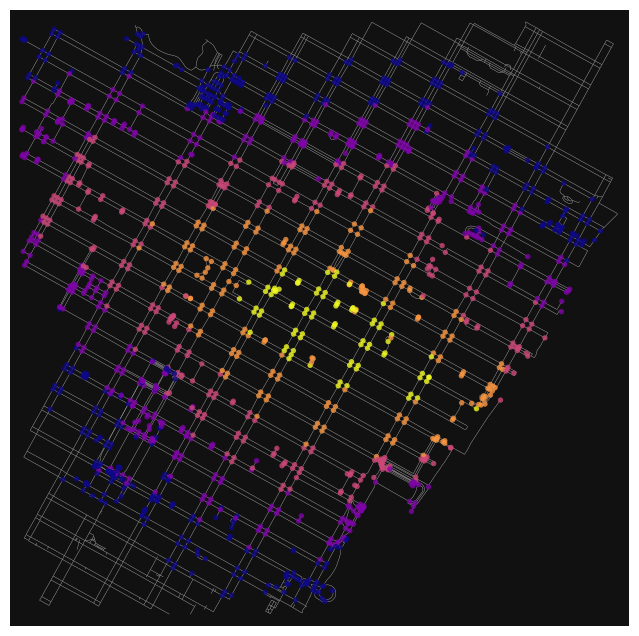
def make_iso_polys(point_network, edge_buff=25, node_buff=50, infill=False):
    isochrone_polys = []
    for trip_time in sorted(trip_times, reverse=True):
        subgraph = nx.ego_graph(point_network, dest, radius=trip_time, distance="time")

        node_points = [
            Point((data["x"], data["y"])) for node, data in subgraph.nodes(data=True)
        ]
        nodes_gdf = gpd.GeoDataFrame({"id": list(subgraph.nodes)}, geometry=node_points)
        nodes_gdf = nodes_gdf.set_index("id")

        edge_lines = []
        for n_fr, n_to in subgraph.edges():
            f = nodes_gdf.loc[n_fr].geometry
            t = nodes_gdf.loc[n_to].geometry
            edge_lookup = point_network.get_edge_data(n_fr, n_to)[0].get(
                "geometry", LineString([f, t])
            )
            edge_lines.append(edge_lookup)

        n = nodes_gdf.buffer(node_buff).geometry
        e = gpd.GeoSeries(edge_lines).buffer(edge_buff).geometry
        all_gs = list(n) + list(e)
        new_iso = gpd.GeoSeries(all_gs).union_all()

        # try to fill in surrounded areas so shapes will appear solid and
        # blocks without white space inside them
        if infill:
            # new_iso = Polygon(new_iso)
            pass
        isochrone_polys.append(new_iso)
    return isochrone_polys


# make the isochrone polygons
isochrone_polys = make_iso_polys(
    point_network, edge_buff=0.0005, node_buff=0, infill=True
)
gdf = gpd.GeoDataFrame(geometry=isochrone_polys)

# plot the network then add isochrones as colored polygon patches
fig, ax = ox.plot.plot_graph(
    point_network,
    show=False,
    close=False,
    edge_color="#999999",
    edge_alpha=0.2,
    node_size=0,
)
gdf.plot(ax=ax, color=iso_colors, ec="none", alpha=0.6, zorder=-1)
plt.show()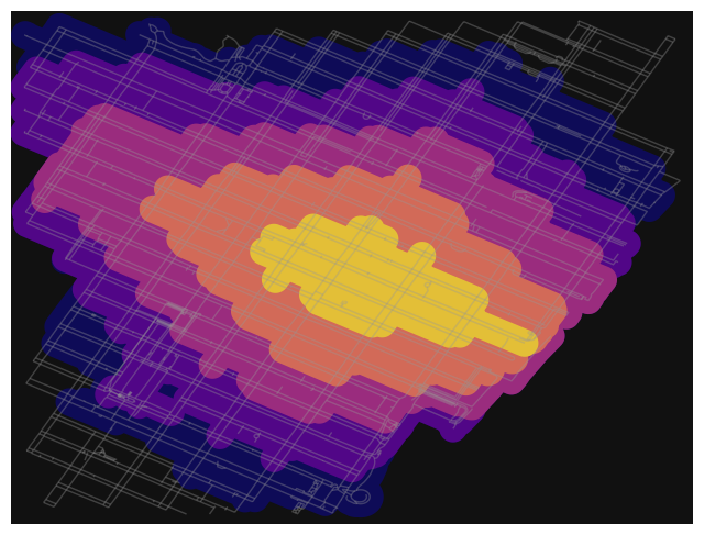
Use grid cells to build and traverse a network
So far, we’ve been able to create networks from a random distribution of points, as well as from the street network of a real-world location. For our final example, let’s explore how we can use a grid of cells to create a network and traverse it. More specifically, we’ll create a grid of hexagons, and then connect each hexagon to its nearest neighbors using the h3 library. H3 was developed by Uber and represents a hierarchical spatial index that uses hexagonal grid cells to partition space. Hexagons are useful for this purpose because they have a number of desirable properties, including uniform adjacency (each hexagon has six neighbors), reduced distortion compared to square grids, and efficient coverage of large areas.
# use H3 grid to create a hexagon around the restaurants
# count the number of restaurants in each hexagon
# use pysal to get adjacency between hexagons
# build new network with hexagons as nodes and their adjacency as edges
# use networkx to find the shortest path between hexagons

# get the H3 hexagonsnet_nodes| y | x | street_count | highway | geometry | |
|---|---|---|---|---|---|
| osmid | |||||
| 42492309 | 40.692089 | -73.963749 | 1 | NaN | POINT (-73.96375 40.69209) |
| 42492312 | 40.692300 | -73.961899 | 1 | NaN | POINT (-73.9619 40.6923) |
| 498897281 | 40.692208 | -73.961884 | 1 | NaN | POINT (-73.96188 40.69221) |
| 504044405 | 40.689861 | -73.964517 | 1 | NaN | POINT (-73.96452 40.68986) |
| 597728150 | 40.681079 | -73.964537 | 1 | traffic_signals | POINT (-73.96454 40.68108) |
| ... | ... | ... | ... | ... | ... |
| 13780532903 | 40.686649 | -73.962374 | 4 | NaN | POINT (-73.96237 40.68665) |
| 13780532905 | 40.686769 | -73.961940 | 1 | NaN | POINT (-73.96194 40.68677) |
| 13780541956 | 40.687427 | -73.960971 | 1 | NaN | POINT (-73.96097 40.68743) |
| 13780541958 | 40.687302 | -73.961260 | 4 | NaN | POINT (-73.96126 40.6873) |
| 13780541959 | 40.687236 | -73.961245 | 1 | NaN | POINT (-73.96125 40.68724) |
1551 rows × 5 columns
Here we are querying the H3 dataset at resolution 9 for each node in our network. You can read more about H3 resolutions here. This will return a unique hexagon id for each point in our network. We will deduplicate these momentarily and create a new dataframe of hexagons.
net_nodes["h3"] = net_nodes.apply(
    lambda x: h3.latlng_to_cell(x.geometry.centroid.y, x.geometry.centroid.x, 9), axis=1
)net_nodes["h3"]osmid
42492309 892a100da83ffff
42492312 892a100da83ffff
498897281 892a100da83ffff
504044405 892a100da8fffff
597728150 892a100da33ffff
...
13780532903 892a100dabbffff
13780532905 892a100dabbffff
13780541956 892a100dabbffff
13780541958 892a100dabbffff
13780541959 892a100dabbffff
Name: h3, Length: 1551, dtype: strWe can use the h3_to_geo_boundary() function to get the polygon geometry of each hexagon, and then populate a new field based on that geometry.
# create hexagons for AOI
net_nodes["geometry"] = net_nodes["h3"].apply(lambda x: (h3.cell_to_boundary(x)))
/var/folders/g5/b592wl6x12s0tx4jfw9f7_j40000gn/T/ipykernel_49295/494313494.py:2: UserWarning: Geometry column does not contain geometry.
net_nodes["geometry"] = net_nodes["h3"].apply(lambda x: (h3.cell_to_boundary(x)))net_nodes["geometry"]osmid
42492309 ((40.694177211706034, -73.9621682675015), (40....
42492312 ((40.694177211706034, -73.9621682675015), (40....
498897281 ((40.694177211706034, -73.9621682675015), (40....
504044405 ((40.6914806830738, -73.96420150874556), (40.6...
597728150 ((40.68350635873867, -73.96602999164979), (40....
...
13780532903 ((40.688899008143295, -73.96196417326604), (40...
13780532905 ((40.688899008143295, -73.96196417326604), (40...
13780541956 ((40.688899008143295, -73.96196417326604), (40...
13780541958 ((40.688899008143295, -73.96196417326604), (40...
13780541959 ((40.688899008143295, -73.96196417326604), (40...
Name: geometry, Length: 1551, dtype: objectUnfortunately H3 returns the polygon vertices in the opposite order that shapely expects them, so we have to reverse the order of the coordinates. We can do so using a list comprehension. While we’re at it, we can also cast the coordinates as a Polygon geometry.
# flip order of coordinates for each tuple
net_nodes["geometry"] = net_nodes["geometry"].apply(
    lambda x: Polygon([(y, x) for x, y in x])
)
We can assign the geometry a crs now that we know it is in lat/lon
net_nodes.crs = "EPSG:4326"net_nodes.crs<Geographic 2D CRS: EPSG:4326>
Name: WGS 84
Axis Info [ellipsoidal]:
- Lat[north]: Geodetic latitude (degree)
- Lon[east]: Geodetic longitude (degree)
Area of Use:
- name: World.
- bounds: (-180.0, -90.0, 180.0, 90.0)
Datum: World Geodetic System 1984 ensemble
- Ellipsoid: WGS 84
- Prime Meridian: GreenwichFinally, we’ll create a new, deduplicated dataframe of hexagons.
h3_lvl_9_cells = net_nodes.dissolve(by="h3").copy().reset_index()h3_lvl_9_cells.boundary.plot()<Axes: >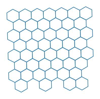
Great, now let’s overlay the hex grid on top of our road network to get a sense of scale and how this new network compares.
ax = h3_lvl_9_cells.boundary.plot(color="black", figsize=(10, 10))
net_edges.plot(
    ax=ax,
    color="black",
    linewidth=0.1,
)
<Axes: >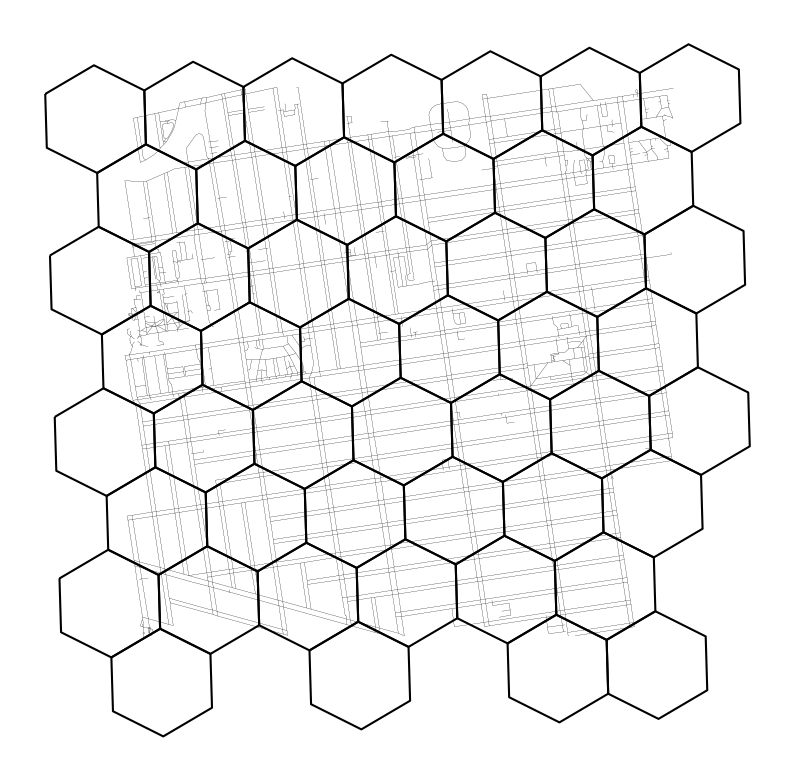
As we can see, the hexagons are fairly small, reasonably appropriate for the scale of our analysis (i.e. traversing city blocks). Next, we will create a network by connecting each hexagon to its six nearest neighbors. While h3 has some native functions to calculate grid adjacency, we will use the more general purpose library libpysal to do so. libpysal is a spatial analysis library that has a number of useful functions, including the ability to calculate spatial weights and relationships between geometries.
We will caalculate a spatial weights matrix using the Queen contiguity method, which considers two polygons to be neighbors if they share a common edge or vertex. This is appropriate for our hexagonal grid, as each hexagon has six neighbors that share edges.
# create an adjacency matrix for the hexagons
w = lps.weights.Queen.from_dataframe(h3_lvl_9_cells)
/var/folders/g5/b592wl6x12s0tx4jfw9f7_j40000gn/T/ipykernel_49295/471419787.py:2: FutureWarning: `use_index` defaults to False but will default to True in future. Set True/False directly to control this behavior and silence this warning
w = lps.weights.Queen.from_dataframe(h3_lvl_9_cells)w.neighbors.items()dict_items([(0, [1, 2, 3]), (1, [0, 2, 3, 6, 10, 15]), (2, [0, 1, 16, 15]), (3, [0, 1, 19, 21, 10]), (4, [16, 13]), (5, [6, 7, 8, 9, 10, 11]), (6, [1, 17, 5, 8, 10, 15]), (7, [32, 5, 38, 8, 11, 28]), (8, [17, 5, 6, 7, 38, 39]), (9, [20, 5, 21, 43, 10, 11]), (10, [1, 3, 5, 6, 21, 9]), (11, [32, 5, 7, 9, 43, 45]), (12, [16, 17, 13, 14, 15]), (13, [16, 4, 12]), (14, [17, 35, 39, 41, 12]), (15, [16, 1, 2, 17, 6, 12]), (16, [2, 4, 12, 13, 15]), (17, [6, 39, 8, 12, 14, 15]), (18, [19, 20, 21, 22, 23]), (19, [18, 3, 21]), (20, [18, 21, 23, 9, 43, 46]), (21, [18, 3, 19, 20, 9, 10]), (22, [18, 23]), (23, [46, 18, 20, 22]), (24, [40, 36, 30]), (25, [26, 36, 37]), (26, [25, 37]), (27, [32, 33, 28, 29, 30, 31]), (28, [32, 38, 7, 40, 27, 30]), (29, [33, 27, 30]), (30, [24, 40, 27, 28, 29]), (31, [32, 33, 27, 44, 45, 47]), (32, [7, 27, 11, 28, 45, 31]), (33, [48, 47, 27, 29, 31]), (34, [35, 36, 37, 38, 39, 40]), (35, [34, 37, 39, 41, 14]), (36, [34, 37, 24, 25, 40]), (37, [34, 35, 36, 25, 26]), (38, [34, 7, 39, 8, 40, 28]), (39, [17, 34, 35, 38, 8, 14]), (40, [34, 36, 38, 24, 28, 30]), (41, [35, 14]), (42, [43, 44, 45, 46]), (43, [20, 9, 42, 11, 45, 46]), (44, [42, 31, 45, 47]), (45, [32, 43, 42, 11, 44, 31]), (46, [42, 43, 20, 23]), (47, [48, 33, 44, 31]), (48, [33, 47])])Just like with the n-nearest neighbors example above, we can use the spatial weights matrix to create a list of neighboring hexagons for each row in our dataframe. We can use dictionary comprehension to create a mapping of each hexagon’s index to its list of neighbors, and then create a graph network from that mapping using networkx.
# get neighbors for each hexagon
neighbors = {k: v for k, v in w.neighbors.items()}neighbors{0: [1, 2, 3],
1: [0, 2, 3, 6, 10, 15],
2: [0, 1, 16, 15],
3: [0, 1, 19, 21, 10],
4: [16, 13],
5: [6, 7, 8, 9, 10, 11],
6: [1, 17, 5, 8, 10, 15],
7: [32, 5, 38, 8, 11, 28],
8: [17, 5, 6, 7, 38, 39],
9: [20, 5, 21, 43, 10, 11],
10: [1, 3, 5, 6, 21, 9],
11: [32, 5, 7, 9, 43, 45],
12: [16, 17, 13, 14, 15],
13: [16, 4, 12],
14: [17, 35, 39, 41, 12],
15: [16, 1, 2, 17, 6, 12],
16: [2, 4, 12, 13, 15],
17: [6, 39, 8, 12, 14, 15],
18: [19, 20, 21, 22, 23],
19: [18, 3, 21],
20: [18, 21, 23, 9, 43, 46],
21: [18, 3, 19, 20, 9, 10],
22: [18, 23],
23: [46, 18, 20, 22],
24: [40, 36, 30],
25: [26, 36, 37],
26: [25, 37],
27: [32, 33, 28, 29, 30, 31],
28: [32, 38, 7, 40, 27, 30],
29: [33, 27, 30],
30: [24, 40, 27, 28, 29],
31: [32, 33, 27, 44, 45, 47],
32: [7, 27, 11, 28, 45, 31],
33: [48, 47, 27, 29, 31],
34: [35, 36, 37, 38, 39, 40],
35: [34, 37, 39, 41, 14],
36: [34, 37, 24, 25, 40],
37: [34, 35, 36, 25, 26],
38: [34, 7, 39, 8, 40, 28],
39: [17, 34, 35, 38, 8, 14],
40: [34, 36, 38, 24, 28, 30],
41: [35, 14],
42: [43, 44, 45, 46],
43: [20, 9, 42, 11, 45, 46],
44: [42, 31, 45, 47],
45: [32, 43, 42, 11, 44, 31],
46: [42, 43, 20, 23],
47: [48, 33, 44, 31],
48: [33, 47]}Here we create a new graph G based on this adjacency matrix.
G = nx.Graph(neighbors)Let’s take a look at the graph- each node ID is plotted on the centroid of each hexagon, and the edges represent the connections between each hexagon and its six neighbors. As before, we can ignore the geographic CRS warning for this example.
# plot the path
ax = h3_lvl_9_cells.plot()
h3_lvl_9_cells.boundary.plot(ax=ax, color="black")

# label cells with their index
for x, y, label in zip(
    h3_lvl_9_cells.geometry.centroid.x,
    h3_lvl_9_cells.geometry.centroid.y,
    neighbors.keys(),
):
    ax.text(x, y, label, fontsize=6)
/var/folders/g5/b592wl6x12s0tx4jfw9f7_j40000gn/T/ipykernel_49295/2249710294.py:7: UserWarning: Geometry is in a geographic CRS. Results from 'centroid' are likely incorrect. Use 'GeoSeries.to_crs()' to re-project geometries to a projected CRS before this operation.
h3_lvl_9_cells.geometry.centroid.x,
/var/folders/g5/b592wl6x12s0tx4jfw9f7_j40000gn/T/ipykernel_49295/2249710294.py:8: UserWarning: Geometry is in a geographic CRS. Results from 'centroid' are likely incorrect. Use 'GeoSeries.to_crs()' to re-project geometries to a projected CRS before this operation.
h3_lvl_9_cells.geometry.centroid.y,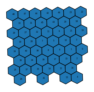
Now we can inspect the adjacency dictionary above and understand how the adjacency is structured. Each key is a hexagon index, and the value is a list of adjacent hexagon indices.
With this in mind, we can use networkx and the shortest_path() function to find the shortest path between two hexagons by passing the graph G and two hexagon indices. Here we are finding the shortest path between hexagon 8 and hexagon 29.
# get the path between two nodes
path = nx.shortest_path(G, 15, 22)
The path is returned as a list of hexagon indices that represent the shortest path between the two input hexagons.
path[15, 1, 3, 19, 18, 22]Finally, let’s visualize the path on top of the hexagon grid. We can use the iloc[...] function to look up the hexagons in path by their indices, and then plot the resulting geometries.
# plot the path
ax = h3_lvl_9_cells.plot()
h3_lvl_9_cells.boundary.plot(ax=ax, color="black")
h3_lvl_9_cells.iloc[path].plot(ax=ax, color="red")

# label cells with their index
for x, y, label in zip(
    h3_lvl_9_cells.geometry.centroid.x,
    h3_lvl_9_cells.geometry.centroid.y,
    neighbors.keys(),
):
    ax.text(x, y, label, fontsize=6)
/var/folders/g5/b592wl6x12s0tx4jfw9f7_j40000gn/T/ipykernel_49295/2962518818.py:8: UserWarning: Geometry is in a geographic CRS. Results from 'centroid' are likely incorrect. Use 'GeoSeries.to_crs()' to re-project geometries to a projected CRS before this operation.
h3_lvl_9_cells.geometry.centroid.x,
/var/folders/g5/b592wl6x12s0tx4jfw9f7_j40000gn/T/ipykernel_49295/2962518818.py:9: UserWarning: Geometry is in a geographic CRS. Results from 'centroid' are likely incorrect. Use 'GeoSeries.to_crs()' to re-project geometries to a projected CRS before this operation.
h3_lvl_9_cells.geometry.centroid.y,
As we can see, the shortest path between the first and second hexagon passes through a number of intermediate hexagons, following the edges of the hexagonal grid. We can imagine cases where this type of grid-based network analysis could be useful.
One thing we didn’t explore as much here is the idea of cost or weight associated with traversing between nodes. In our street network example above, we used the length of each street segment as the weight for calculating the shortest path. We could just as easily assign other weights, such as travel time, elevation change, degree of sun exposure, etc. Think about the possibilities!