02: Geoprocessing

Goals¶

This notebook will walk through some common geoprocessing tasks using geopandas. These operations include:

• reprojecting data
• using a mask to clip data
• performing a spatial join
• performing an attribute join
• dissolving data
• unioning data
• writing functions to calculate new attributes

Together, these operations form the basis of many geospatial analyses. These tools are used to explore our datasets and the relationships between them, a common first step in any geospatial analysis.

Import libraries¶

Now we can run the function to set the default settings for this notebook.

Import datasets¶

As you may have noticed in the previous notebook, Pluto is a huge dataset that takes a long time to load. In geopandas, you can use the where=... argument to load only a subset of the data. This is useful when you want to work with a smaller area or a specific set of features. In this case, we will focus only on tax lots within Brooklyn’s community district 7 (where="CD = 307"). This will significantly speed up the loading process (and takes out the additional step of filtering the data later).

To get to know CD 307 a bit better, let’s check the distribution of land use types in this community district.

With this trick, we are able to load only a subset of lots that we are interested in. Next we will load in building foorprints, but that dataset does not have the CD attribute to be able to filter by. Instead, we will use a geometric filter based on the bounds of our tax lot geodataframe.

We can get the “total bounds” of our dataset using the total_bounds property of the GeoDataFrame.

The “total bounds” is an array of the minimum and maximum x and y coordinates of the geometries in the GeoDataFrame- it is a minimum bounding rectagle for the entire dataset.

Let’s visually inspect the bounds of our tax lots.

As an array, this isn’t much use to us yet- we need to convert it to a polygon object to be able to use it as a filter. Note that we are also passing the crs argument to ensure that the polygon is in the same coordinate reference system as our tax lots (and is aware of that fact).

Now we can see that the bounds are a polygon that covers the entire area of interest.

If we plot both datasets together and zoom in, you can see that the bounding polygon exactly matches the extent of the tax lots.

Aligning dataset projections¶

We saw in the previous exercise that the buildings geojson file has a CRS of EPSG:4326, which is WGS84. Unlike desktop GIS software, GeoPandas does not reproject on-the-fly; as such, we need to explicitly align projections between our datasets to be able to work with them together.

You can check a dataset’s CRS (Coordinate Reference System) with the .crs attribute. If this returns None, the dataset does not have a CRS defined and you can set it with the .set_crs([crs-here]) method or [dataset].crs = [crs-here].

To be able to use our bounds polygon to filter the building footprints dataset, we’ll need to create a copy of the bounds that are in the right coordinate system. we can create a copy and use the to_crs() method to convert into the proper system

We can confirm that the CRS has changed by checking the CRS attribute again.

Similar to the attribute filter we used previously to only load tax lots in CD 307, we can use a spatial filter to only load building footprints that intersect with our bounds polygon using the mask=... argument in our input statement.

Now let’s visually inpect the buildings in the area of interest.

So, we are able to successfully read in the building footprints within thd study area and plot them- however, we see that there are also point representations of buildings along with the expected polygon shapes. Let’s exclude point type features to be able to work specifically with polygons:

Combine building footprints and tax lot data¶

To combine our building footprints with tax lots, we will compare the spatial relations between the two geometries. There are a few quirks to keep in mind:

• in some cases, buildings can cross between tax lots, leaving open the possibility that there are multiple matching tax lots for a single building footprint.
• in other cases, a building footprint may not intersect with any tax lot, such as when a building is on a sidewalk or in a park.

Because of these quirks, we will use a representation of the building footprints that is a representative point of the polygon, which is a single point representation of the building footprint. This will allow us to match each building footprint to a single tax lot.

It’s worth mentioning that the buildings do have join attributes that we could use to join the two datasets (mpluto_bbl and base_bbl), but for the purposes of this exercise, we will focus on the spatial join.

Note:
The representative_point() method is a way to get a point that is guaranteed to be within the polygon, even if the polygon is complex or has holes. This is useful for matching geometries that may not overlap perfectly. This is a related concept to the centroid method, which returns the center point of the polygon, but the representative point is guaranteed to be within the polygon.

To illustrate this point, we’ll take a random building footprint using the sample() method. We’ll look at it’s simplified geometry using the boundary property, along with the representative point of the polygon.

Okay, now that we understand the concept of representative points, let’s generate one for each building footprint in our dataset. We’ll then set this column as the geometry of the GeoDataFrame so that we can use it for spatial operations (while still keeping the original geometry for reference).

Let’s take a look- we can see two geometry columns now, one for the original building footprint and one for the representative point.

Of course, there are plenty of cases where there are multiple buildings on a single tax lot. We can compare the number of unique tax lot ids with the number of buildings / building IDs to get a sense of this relationshp:

Perform spatial join¶

Now we will use the spatial join operation to join the building footprints to the tax lots based on the relationship between the representative points and lot polygons. The spatial join is a fundamental operation in GIS that allows us to combine attributes from two different datasets based on their spatial relationship. Read more about geopandas’ implementation of spatial joins in the documentation, and note that some of the directives have changed between recent versions.

Here we take a subset of attributes of the buildings layer, denoted in the double brackets [[...]] and use the sjoin() method to join to the tax lots layer.

We are performing an inner join, matching overlapping features between the two datasets, vs. an outer, right, or left join. We are also using the spatial predicate within to specify what kind of spatial relationship we want to use as the basis of the join.

Let’s try a different approach- we can use a similar function, sjoin_nearest() to join features to the nearest feature in the target dataset. In this example, we are performing a left join, which means we are keeping all features in the input dataset, but we need to keep in mind that there may be cases where multiple input features are closest to a target (tax lot) feature. There’s an optional argument for the function, exclusive which defaults to False, which would allow us to prevent duplicate matches.

We will pass in an additional optional argument, distance_col, which will calculate and record the distance from our input features from the matching target feature. This is important as we explore the spatial relationship between our datasets.

We can plot the distance field to visualize how far each input feature is from a target feature. What do you notice?

Now let’s visualize our building points on top of our tax lots

Merge back with footprints¶

Now that we’ve associated each tax lot with every building’s representative point, we can merge back with the input footprint geometry to be able to represent the data using footprints.

In the below example, we are chaining a few different operations together:

• using the drop() function to get rid of the rep_pt column, which we no longer need
• using the merge() function to merge the data we do want to keep with our previous building footprints dataset, making sure to only keep the building footprints with matches (based on the left directive)

We need to cast our new dataset explicitly as a geodataframe for geopandas to be able to recognize that geometry is a special column.

... and we’ll borrow the colormap we created in the first notebook here to be able to produce a consistent representation of land uses on a per-lot and building basis

Similarly, we will convert the hex code-based cmap to the RGB-type representation that lonboard needs for visualizing

Let’s visually inspect the relationships between land use and color columns just to make sure things are mapped properly.

Now let’s use lonboard to plot the output in 3D. we should be able to see each building shaded in the color that represents a land use based off it’s spatial relationship with tax lots from the previous steps. Because each building footprint has an estimated height field (heightroof), we can use that as the extrude height for each feature.

Across the above steps, we’ve witnessed how the spatial relationships between different datasets can be messy- items can overlap with multiple features, or not overlap with any features! At every step, we need to investigate how and to what degree our data matches. Thankfully, as we saw above, these datasets do share an attribute that can be used to connect: the bbl identifier, which stands for borough block lot.

We will use this shared attribute as the basis for a join in the next steps.

Performing attribute joins¶

Remember that we brought in the building footprints layer based on a mask, and that the building footprints’ extent exceeds that of the community district we are interested in. We can confirm this by looking at the number of unique mpluto_bbl entries vs the number of records in our cb_307 dataset.

Before we merge, together, we need to confirm that the BBLs are encoded as the same data type- as we see below, the building footprints dataset encodes the BBLs as O or objects (i.e. as strings) and the tax lot dataset encodes them as float64 numbers. We’ll need to convert one or the other to be able to join them together

We can convert the building mpluto_bbl field as floats to match the tax lot dataset. We could just as easily go in the opposite direction and convert the tax lot dataset to objects instead (e.g. ...astype(str))

Now we can merge the datasets together- in cases where the join field is not the same, you have to specify left_on=... and right_on=... instead of just on=.... Since we are only interested in cases where the records overlap (i.e. in CB 307), we will do an inner join. In this particular case, that’s the same as doing a right join.

We will also use the suffixes attribute to properly name fields that exist in both datasets to not get confused later. (The default behavior is to append _x and _y to matching columns).

As you can see, joining based on attributes can be a more straightforward process than the various operations we had to conduct for the spatial join. Now we can compare these results against our previous spatial join results. At a high level, we can see (in the next cell) that the dataframes are not the same length, meaning that at some point, certain features are dropped (or not) in different ways between the different datasets. What do you think those points of difference are?

They don’t match! How close are they?

Not bad- but there are three buildings that our spatial join did not pick up that our attribute join did. Let’s investigate.

Let’s compare the two datasets. Below we’ll plot the longer, more complete list of buildings generated through the attribute join vs. the buildings that do not match between the two. We will use the selection logic in square brackets to perform this selection.

We are selecting from the dataset using the conditions in the square brackets. The ~ operator means not- so we are selecting the reverse of the following statement: bldgs_w_lot_attrib.globalid.isin(bldgs_w_lot_gdf.globalid). This statement looks for cases where the global building id from the attribute join bldgs_w_lot_attrib dataset is in the list of the spatial join dataset’s (bldgs_w_lot_gdf) global ids. Because we start this filter off with the ~, we are asking for cases where IDs are in the attribute join dataset, but not the spatial join dataset.

Filter statements like this can be written in a number of different ways, so be sure to mind each part of the statement as you construct your filter.

Now let’s look at the inverse and create a new dataframe which includes only the three missing buildings. We’ll use a similar selection logic as before. We’ll then confirm that there are three missing buildings in our dataframe.

To be able to visually inspect those missing buildings against our other joined buildings, we’ll have to clean up our joined dataset: because both the lot and the building dataset contained geometry fields, we now have geometry_lot and geometry_bldg. We need to clarify which we want to use. We have a few options:

• we can create a new column named geometry and set it to the value of geometry_bldg, and then set the geodataframe’s geometry column to that using set_geometry
• we can just set the geometry column to be geometry_bldg.

There is no right or wrong choice here- for the sake of brevity we’ll directly set the geometry column.

Map the missing buildings¶

Map the missing buildings and zoom around to find where they are and what kind of spatial relationship(s) they have with the tax lot dataset.

So we can see that there are three cases where buildings are associated with lots, even if their representative point (or entire geometry) fall outside of the actual polygon.

Dissolve¶

A common geoprocessing operation is to dissolve features based on a shared attribute. This is useful when you want to aggregate data to a higher level of geography, such as aggregating tax lots to blocks or neighborhoods, or based on a shared attribute. This is similar to the groupby() function in pandas, but it also merges the geometries of the features that are being grouped together.

In this case, we will dissolve lots based on the OwnerName field: we will merge all lots that share the same owner into a single polygon. This is useful for understanding the extent of land owned by a particular entity.

You can read more about the dissolve() function in the geopandas documentation.

At the most basic level, you can dissolve all the geometry together into a single feature by not passing any arguments to the dissolve() function- however, this may not be very useful on its own. You can pass the by=... argument to specify which attribute to dissolve by (very similar to the groupby() function in pandas).

You can also specify how you want to treat other attributes in the dataset using the aggfunc=... argument. By default, this is set to first, which means that for each group of features being dissolved, the first value of each attribute will be kept. You can also use other aggregation functions such as sum, mean, min, max, etc. You can also pass a dictionary to specify different aggregation functions for different attributes. In the below example, we will pass a dictionary with two entries:

• we want to get a list of all of the different LandUse types for each owner (what kinds of land do they own?)
• we want to get the sum of the LotArea field for each owner (how much land do they own in total?)

Finally, we use the as_index=False argument to ensure that the OwnerName field is kept as a column in the output dataframe, rather than being set as the index. We could instead use reset_index() after the dissolve operation to achieve the same effect.

Let’s take a look at the top ten owners with the greatest total lot area.

And now let’s map the results using the OwnerName field to color the dissolved polygons.

Take a look at the results- what do you notice? It’s clear from the above that the results are limited by the availability of complete data.

Intersect / Difference¶

Next we’ll perform additional geometric operations to identify the portions of tax lots that are not covered by buildings. This workflow demonstrates how to create a new dataset based on existing inputs.

To begin, we’ll choose a random block within CB 307.

Now we’ll select the blocks and building footprints that match the randomly selected block, and will create new dataframes for each.

We can plot those to visually inspect the sampled block, lots, and building footprints.

Next we can identify the portions of the block that are not buildings by calculating the difference between the lots and the buildings. We will use the unary_union property of the buildings dataframe, which represents a union of all geometries in the dataframe. It is essentially a shortcut to a dissolve of all geometries in a dataframe.

With these chained commands, we will return the area of each tax lot that is not a building.

We can plot the results to confirm that each lot still exists as its own feature (blue with black outlines) and are separate from the orange building polygons. Note that in some cases, lots may be split into two distinct areas, making them MultiPolygons.

We could use this new dataset to calculate the lot coverage of each lot, which could be useful in a soft site analysis (continued below). Next we will explore another means of calculating lot coverage by unioning features instead of taking the intersection.

Union¶

We’ll continue using the sample block we identified above. We’ll start by calculating the lot area of each lot in our sample.

Now we’ll perform a union between the lots and the building footprints. A union, like the difference performed above, is a kind of overlay method that we can apply between multiple dataframes. (For more information on other overlay methods, check out the documentation). The union operation retains all geometry of the input layers, as well as the attributes of each based on the overlap.

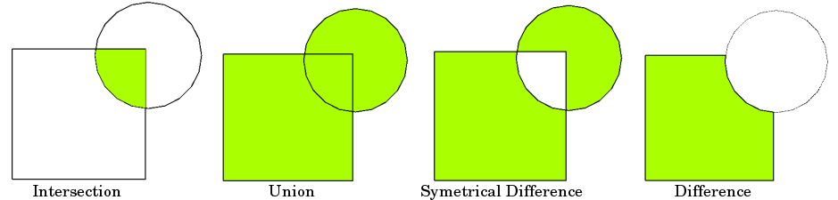
Source: QGIS Documentation via Geopandas docs

A union would take the following input:

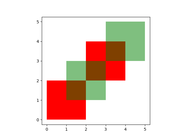
and produce the following output:

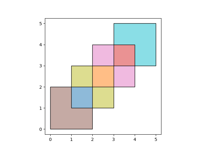
A union will produce features that have geometry entries (based on the union operation), as well as attributes from both input datasets so long as there is coverage of that dataset. In our example, there will be full attributes of both datasets for the portion of the lots that are buildings, but the other portions of lots will not have attributes from the buildings dataset.

We can illustrate that point by mapping the output layer. In the below example, we filter for cases where the globalid (which is associated with the buildings dataset) is null (.isna()) in grey. Cases where the globalid is not null are red.

We can also plot based on a shared attribute to demonstrate that both portions of the lots (building and non-building) are part of the same lot. Plotting the boundary separately confirms that each segment of the building/lot combination is in fact a separate feature.

Finally, we can create a new attribute field that represents the percent of the lot that is covered by a building as discussed above. The below operation uses a lambda function, which is a way to iterate through a dataframe and perform a calculation on each row (or column, based on the axis=... argument). The function can be understood as follows:

• lambda x: ... axis=1 for each row (x, based on the 1 axis value), perform the following operation
• ((x.geometry.area / x.lot_area)*100...): take the geometry of each piece of the unioned dataframe, calculate the area, divide it by the lot area (which we calculated above, pre-union), and multiply by 100 to get a percentage
• if type(x.globalid) == str else -1: only do this for the input features that are pieces of buildings (e.g. they have a globalid), otherwise return a placeholder value of -1. This number is negative on purpose so it is easy to filter out, but you could also use None or NaN if you prefer.

As you can see, we can perform a multi-step operation using a lambda function. For more complex operations, it makes sense to write standalone functions for legibility- we’ll demonstrate that in the following section. There is no hard rule for legibility vs. brevity (i.e. lambda vs standalone functions), so use your best judgement. What’s important is that you or your user understand what the code is doing.

Now let’s plot and see the percentage of each lot that is covered by buildings. This could be expressed in a number of different ways (e.g. at the lot level) but we can get a sense of the utility of the union operation.

Creating new attributes¶

In this example, we’ll develop a function that indicates whether a site is a “soft site” or not. A “soft site” is a site that meets certain criteria for redevelopment. The factors below represent just a few of the considerations that are often taken to determine whether a site may be a good candidate for redevelopment, but this is a simplistic example case to illustrate a point rather than a firm ruleset.

Because we are considering a few different factors, we will write a new function vs. chaining criteria together in a lambda function (although you could use the same kind of syntax above to perform the same work).

There are several important components to consider.

def [function_name]([input_args...]): The instantiation of the function is important. We are defining (def) a new function, giving it a name (in this case, is_soft_site), and indicating that there are two possible input arguments: r, which is a common shorthand for a row in a dataset, and the optional argument threshold. This is optional and comes with a default value of 0.33, meaning that if a user doesn’t specify a threshold, 0.33 will be used. You could imagine other cases where required or optional arguments might be useful!

if (...): return 1 else: return 0 This is the part of the function that is evaluating properties of our input r based on it’s properties. We can see the evaluation of its BuiltFAR compared to the lot’s ResidFAR (allowed residential FAR) times the threshold set here. We are determining whether the site is built less than or equal to 33% of the allowable residential FAR.

We then evaluate the lot area, existing land use, and whether there is available residential FAR at all to indicate that yes, this is a soft site, or no, it is not. The return statements are what pass that information back to us: if those conditions are met, we get a 1, otherwise a 0.

Functions don’t necessarily have to return anything, but in this case we will be using this logic to create a new field and so want to be sure that something is always returned.

We can invoke the function using the apply() method- here we pass in the function name, and specify that we want to apply the function to each row (axis=1) vs each column (axis=0) of our table.

If we wanted to pass in a threshold value, we could pass in a tuple of arguments: ...apply(is_soft_site, axis=1, args=(0.5,)) which is then passed in as a different threshold. Part of the point of providing these optional attributes is to make it easier for you / your users to make changes quickly- in a more complex example you might also have arguments for your lot area thresholds, the land uses that are off limits, etc.

Now let’s check how many soft sites we have in the neighborhood based on the criteria we defined above. Because we use 1/0 values to distinguish soft sites from not, we can use the value_counts() method to get a quick overview of the number of soft sites in the neighborhood.

Now let’s create a quick map to see where our soft sites are. What do you notice about the distribution of sites?